Mahotas - 分水嶺演算法

在影像處理中，分水嶺演算法用於影像分割，這是將影像分割成不同區域的過程。分水嶺演算法尤其適用於分割具有不均勻區域或邊界不明確的區域的影像。

分水嶺演算法的靈感來自於水文學中的分水嶺概念，水從高處流向低處，沿山脊流淌，直到到達最低點，形成盆地。

同樣，在影像處理中，該演算法將影像的灰度值視為地形表面，其中高強度值代表峰值，低強度值代表谷值。

分水嶺演算法的工作原理

以下是分水嶺演算法在影像處理中工作原理的概述：

• 影像預處理：將輸入影像轉換為灰度影像（如果它不是灰度影像）。執行任何必要的預處理步驟，例如噪聲去除或平滑處理，以改善結果。

• 梯度計算：計算影像的梯度以識別強度變化。這可以透過使用梯度運算元（例如Sobel運算元）來突出邊緣。

• 標記生成：識別將用於啟動分水嶺演算法的標記。這些標記通常對應於影像中感興趣的區域。

  它們可以由使用者手動指定，也可以根據某些標準（例如區域性最小值或聚類演算法）自動生成。

• 標記標記：使用不同的整數值標記影像中的標記，表示不同的區域。

• 分水嶺變換：使用標記的標記計算影像的分水嶺變換。這是透過模擬洪水過程來完成的，其中強度值從標記傳播並填充影像，直到它們在不同區域的邊界處相遇。

  結果是一個灰度影像，其中區域之間的邊界被突出顯示。

• 後處理：分水嶺變換可能會產生過度分割的區域。可以應用後處理步驟（例如合併或平滑）來細化分割結果並獲得最終的分割影像。

Mahotas中的分水嶺演算法

Mahotas庫沒有直接應用傳統分水嶺演算法於影像的函式。但是，Mahotas提供了一種類似的技術，稱為條件分水嶺，我們將在後面的章節中詳細探討和討論。

為了更好地理解傳統的分割演算法，讓我們來看一個使用cv2庫進行影像分割的例子。

示例

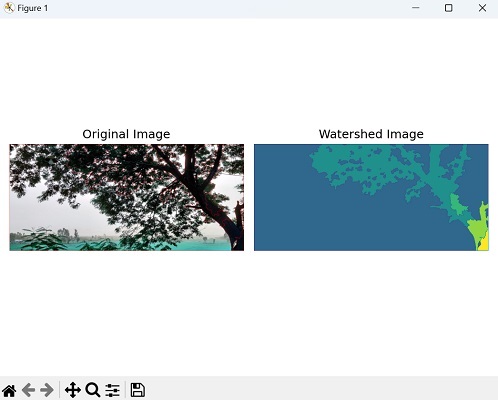
在下面的示例中，我們應用Otsu閾值化、形態學運算和距離變換來預處理影像並獲得前景和背景區域。

然後，我們使用基於標記的分水嶺分割來標記區域，並在分割影像中將邊界標記為紅色。

import cv2
import numpy as np
from matplotlib import pyplot as plt
image = cv2.imread('tree.tiff')
# Convert the image to grayscale
gray = cv2.cvtColor(image, cv2.COLOR_BGR2GRAY)
# Apply Otsu's thresholding
_, thresh = cv2.threshold(gray, 0, 255, cv2.THRESH_BINARY_INV +
cv2.THRESH_OTSU)
# Perform morphological opening for noise removal
kernel = np.ones((3, 3), np.uint8)
opening = cv2.morphologyEx(thresh, cv2.MORPH_OPEN, kernel, iterations=2)
# Perform distance transform
dist_transform = cv2.distanceTransform(opening, cv2.DIST_L2, 5)
# Threshold the distance transform to obtain sure foreground
_, sure_fg = cv2.threshold(dist_transform, 0.7 * dist_transform.max(), 255, 0)
sure_fg = np.uint8(sure_fg)
# Determine the sure background region
sure_bg = cv2.dilate(opening, kernel, iterations=3)
# Determine the unknown region
unknown = cv2.subtract(sure_bg, sure_fg)
# Label the markers for watershed
_, markers = cv2.connectedComponents(sure_fg)
markers = markers + 1
markers[unknown == 255] = 0
# Apply watershed algorithm
markers = cv2.watershed(image, markers)
image[markers == -1] = [255, 0, 0]
# Create a figure with subplots
fig, axes = plt.subplots(1, 2, figsize=(7,5 ))
# Display the original image
axes[0].imshow(image)
axes[0].set_title('Original Image')
axes[0].axis('off')
# Display the watershed image
axes[1].imshow(markers)
axes[1].set_title('Watershed Image')
axes[1].axis('off')
# Adjust the layout and display the plot
plt.tight_layout()
plt.show()

輸出

以下是上述程式碼的輸出：