Mahotas - Bernsen 區域性閾值化

Bernsen 區域性閾值化是一種用於將影像分割成前景和背景區域的技術。它利用區域性鄰域的強度變化為影像中的每個畫素分配閾值。

區域性鄰域的大小使用視窗確定。較大的視窗大小在閾值化過程中考慮更多的鄰域畫素，從而在區域之間建立更平滑的過渡，但會去除更精細的細節。

另一方面，較小的視窗大小可以捕獲更多細節，但可能容易受到噪聲的影響。

Bernsen 區域性閾值化與其他閾值化技術的區別在於，Bernsen 區域性閾值化使用動態閾值，而其他閾值化技術使用單個閾值來分離前景和背景區域。

Mahotas 中的 Bernsen 區域性閾值化

在 Mahotas 中，我們可以使用 **thresholding.bernsen()** 和 **thresholding.gbernsen()** 函式將 Bernsen 區域性閾值化應用於影像。這些函式建立一個固定大小的視窗，並計算視窗內每個畫素的區域性對比度範圍以分割影像。

區域性對比度範圍是視窗內的最小和最大灰度值。

然後將閾值計算為最小和最大灰度值的平均值。如果畫素強度高於閾值，則將其分配給前景（白色），否則將其分配給背景（黑色）。

然後視窗在影像上移動以覆蓋所有畫素，以建立二值影像，其中前景和背景區域根據區域性強度變化進行分離。

mahotas.tresholding.bernsen() 函式

mahotas.thresholding.bernsen() 函式以灰度影像作為輸入，並對其應用 Bernsen 區域性閾值化。它輸出一個影像，其中每個畫素被分配 0（黑色）或 255（白色）的值。

前景畫素對應於影像中具有相對較高強度的區域，而背景畫素對應於影像中具有相對較低強度的區域。

語法

以下是 mahotas 中 bernsen() 函式的基本語法：

mahotas.thresholding.bernsen(f, radius, contrast_threshold, gthresh={128})

其中，

**f** - 輸入灰度影像。
**radius** - 每個畫素周圍視窗的大小。
**contrast_threshold** - 區域性閾值。
**gthresh（可選）** - 全域性閾值（預設為 128）。

示例

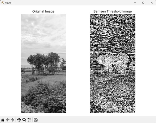
以下示例顯示了使用 mh.thresholding.bernsen() 函式將 Bernsen 區域性閾值化應用於影像。

import mahotas as mh
import numpy as np
import matplotlib.pyplot as mtplt
# Loading the image
image = mh.imread('nature.jpeg')
# Converting it to grayscale
image = mh.colors.rgb2gray(image)
# Creating Bernsen threshold image
threshold_image = mh.thresholding.bernsen(image, 5, 200)
# Creating a figure and axes for subplots
fig, axes = mtplt.subplots(1, 2)
# Displaying the original image
axes[0].imshow(image, cmap='gray')
axes[0].set_title('Original Image')
axes[0].set_axis_off()
# Displaying the threshold image
axes[1].imshow(threshold_image, cmap='gray')
axes[1].set_title('Bernsen Threshold Image')
axes[1].set_axis_off()
# Adjusting spacing between subplots
mtplt.tight_layout()
# Showing the figures
mtplt.show()

輸出

以下是上述程式碼的輸出：

mahotas.thresholding.gbernsen() 函式

mahotas.thresholding.gbernsen() 函式也對輸入灰度影像應用 Bernsen 區域性閾值化。

它是 Bernsen 區域性閾值化演算法的廣義版本。它輸出一個分割影像，其中每個畫素被分配 0 或 255 的值，具體取決於它是背景還是前景。

gbernsen() 和 bernsen() 函式的區別在於，gbernsen() 函式使用結構元素來定義區域性鄰域，而 bernsen() 函式使用固定大小的視窗來定義畫素周圍的區域性鄰域。

此外，gbernsen() 根據對比度閾值和全域性閾值計算閾值，而 bernsen() 僅使用對比度閾值來計算每個畫素的閾值。

語法

以下是 mahotas 中 gbernsen() 函式的基本語法：

mahotas.thresholding.gbernsen(f, se, contrast_threshold, gthresh)

其中，

**f** - 輸入灰度影像。
**se** - 結構元素。
**contrast_threshold** - 區域性閾值。
**gthresh（可選）** - 全域性閾值。

示例

在這個例子中，我們使用 mh.thresholding.gbernsen() 函式將廣義 Bernsen 區域性閾值化應用於影像。

import mahotas as mh
import numpy as np
import matplotlib.pyplot as mtplt
# Loading the image
image = mh.imread('nature.jpeg')
# Converting it to grayscale
image = mh.colors.rgb2gray(image)
# Creating a structuring element
structuring_element = np.array([[0, 0, 0],[0, 0, 0],[1, 1, 1]])
# Creating generalized Bernsen threshold image
threshold_image = mh.thresholding.gbernsen(image, structuring_element, 200,
128)
# Creating a figure and axes for subplots
fig, axes = mtplt.subplots(1, 2)
# Displaying the original image
axes[0].imshow(image, cmap='gray')
axes[0].set_title('Original Image')
axes[0].set_axis_off()
# Displaying the threshold image
axes[1].imshow(threshold_image, cmap='gray')
axes[1].set_title('Generalized Bernsen Threshold Image')
axes[1].set_axis_off()
# Adjusting spacing between subplots
mtplt.tight_layout()
# Showing the figures
mtplt.show()

輸出

上述程式碼的輸出如下：

使用均值的 Bernsen 區域性閾值化

我們可以使用畫素強度的平均值作為閾值來應用 Bernsen 區域性閾值化。它指的是影像的平均強度，透過將所有畫素的強度值求和，然後除以畫素總數來計算。

在 mahotas 中，我們可以首先使用 numpy.mean() 函式找到所有畫素的平均畫素強度。然後，我們定義一個視窗大小以獲取畫素的區域性鄰域。

最後，我們將平均值設定為閾值，將其傳遞給 bernsen() 或 gbernsen() 函式的 **contrast_threshold** 引數。

示例

這裡，我們正在對影像應用 Bernsen 區域性閾值化，其中閾值是所有畫素強度的平均值。

import mahotas as mh
import numpy as np
import matplotlib.pyplot as mtplt
# Loading the image
image = mh.imread('nature.jpeg')
# Converting it to grayscale
image = mh.colors.rgb2gray(image)
# Calculating mean pixel value
mean = np.mean(image)
# Creating bernsen threshold image
threshold_image = mh.thresholding.bernsen(image, 15, mean)
# Creating a figure and axes for subplots
fig, axes = mtplt.subplots(1, 2)
# Displaying the original image
axes[0].imshow(image, cmap='gray')
axes[0].set_title('Original Image')
axes[0].set_axis_off()
# Displaying the threshold image
axes[1].imshow(threshold_image, cmap='gray')
axes[1].set_title('Bernsen Threshold Image')
axes[1].set_axis_off()
# Adjusting spacing between subplots
mtplt.tight_layout()
# Showing the figures
mtplt.show()

輸出

執行上述程式碼後，我們將獲得以下輸出：

列印頁面