Mahotas - Sobel 邊緣檢測

---

---

Sobel 邊緣檢測是一種用於識別影像中邊緣的演算法。邊緣代表不同區域之間的邊界。它的工作原理是計算每個畫素的影像強度梯度。

簡單來說，它測量畫素值的改變以確定高變化區域，這些區域對應於影像中的邊緣。

Mahotas 中的 Sobel 邊緣檢測

在 Mahotas 中，我們可以使用 **mahotas.sobel()** 函式來檢測影像中的邊緣。

Sobel 函式使用兩個單獨的濾波器，一個用於水平變化 (Gx)，另一個用於垂直變化 (Gy)。

這些濾波器透過卷積與影像的畫素值應用於影像。這計算了水平和垂直方向的梯度。

一旦獲得兩個方向的梯度，Sobel 函式就會將它們組合起來計算每個畫素的整體梯度幅度。

這是使用勾股定理完成的，它計算水平和垂直梯度的平方和的平方根。

$$\mathrm{M\:=\:\sqrt{(Gx^{2}\:+\:Gy^{2})}}$$

影像的最終梯度幅度 (M) 表示原始影像中邊緣的強度。較高的值表示較強的邊緣，而較低的值對應於較平滑的區域。

mahotas.sobel() 函式

mahotas.sobel() 函式接收灰度影像作為輸入，並返回二值影像作為輸出，其中邊緣使用 Sobel 邊緣檢測演算法計算。

結果影像中的白色畫素表示邊緣，而黑色畫素表示其他區域。

語法

以下是 Mahotas 中 sobel() 函式的基本語法：

mahotas.sobel(img, just_filter=False)

其中：

• **img** - 輸入灰度影像。

• **just_filter (可選)** - 一個標誌，用於指定是否對濾波後的影像進行閾值化（預設值為 false）。

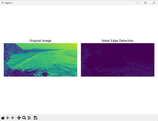
示例

在下面的示例中，我們使用 Sobel 邊緣檢測演算法來使用 mh.sobel() 函式檢測邊緣。

import mahotas as mh
import numpy as np
import matplotlib.pyplot as mtplt
# Loading the image
image = mh.imread('sea.bmp')
# Converting it to grayscale
image = mh.colors.rgb2gray(image)
# Applying sobel gradient to detect edges
sobel = mh.sobel(image)
# Creating a figure and axes for subplots
fig, axes = mtplt.subplots(1, 2)
# Displaying the original image
axes[0].imshow(image)
axes[0].set_title('Original Image')
axes[0].set_axis_off()
# Displaying the edges
axes[1].imshow(sobel)
axes[1].set_title('Sobel Edge Detection')
axes[1].set_axis_off()
# Adjusting spacing between subplots
mtplt.tight_layout()
# Showing the figures
mtplt.show()

輸出

以下是上述程式碼的輸出：

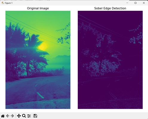
未進行閾值化的輸出影像

我們還可以不進行閾值化輸出影像來執行 Sobel 邊緣檢測演算法。閾值化是指透過將畫素分類為前景或背景來將影像轉換為二值影像。

轉換是透過將畫素的強度值與閾值（固定）值進行比較來實現的。

在 Mahotas 中，sobel() 函式中的 **just_filter** 引數決定是否對輸出影像進行閾值化。我們可以將此引數設定為“True”以防止對輸出影像進行閾值化。

如果過濾器設定為“False”，則會對輸出影像進行閾值化。

示例

在下面提到的示例中，我們在使用 Sobel 邊緣檢測演算法時沒有對輸出影像進行閾值化。

import mahotas as mh
import numpy as np
import matplotlib.pyplot as mtplt
# Loading the image
image = mh.imread('sun.png')
# Converting it to grayscale
image = mh.colors.rgb2gray(image)
# Applying sobel gradient to detect edges
sobel = mh.sobel(image, just_filter=True)
# Creating a figure and axes for subplots
fig, axes = mtplt.subplots(1, 2)
# Displaying the original image
axes[0].imshow(image)
axes[0].set_title('Original Image')
axes[0].set_axis_off()
# Displaying the edges
axes[1].imshow(sobel)
axes[1].set_title('Sobel Edge Detection')
axes[1].set_axis_off()
# Adjusting spacing between subplots
mtplt.tight_layout()
# Showing the figures
mtplt.show()

輸出

執行上述程式碼後，我們將得到以下輸出：

在閾值影像上

Sobel 邊緣檢測也可以在閾值影像上執行。閾值影像是一個二值影像，其中畫素被分類為前景或背景。

前景畫素為白色，用值 1 表示，而背景畫素為黑色，用值 0 表示。

在 Mahotas 中，我們首先使用任何閾值化演算法對輸入影像進行閾值化。讓我們假設Bernsen 閾值化演算法。這可以透過在灰度影像上使用 mh.thresholding.bernsen() 函式來完成。

然後，我們應用 Sobel 邊緣檢測演算法來檢測閾值影像的邊緣。

示例

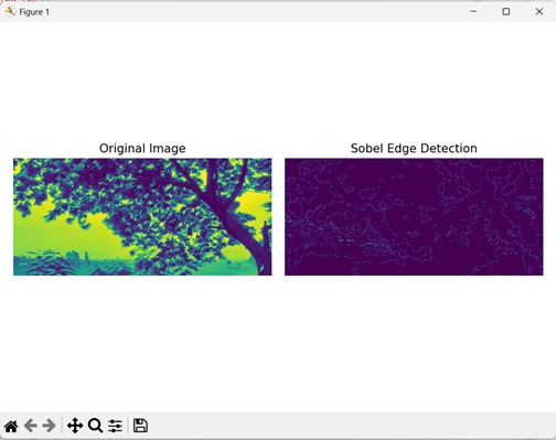
在這裡，我們正在使用 Sobel 邊緣檢測演算法在閾值影像上檢測影像的邊緣。

import mahotas as mh
import numpy as np
import matplotlib.pyplot as mtplt
# Loading the image
image = mh.imread('tree.tiff')
# Converting it to grayscale
image = mh.colors.rgb2gray(image)
# Applying threshold on the image
threshold_image = mh.thresholding.bernsen(image, 17, 19)
# Applying sobel gradient to detect edges
sobel = mh.sobel(threshold_image)
# Creating a figure and axes for subplots
fig, axes = mtplt.subplots(1, 2)
# Displaying the original image
axes[0].imshow(image)
axes[0].set_title('Original Image')
axes[0].set_axis_off()
# Displaying the edges
axes[1].imshow(sobel)
axes[1].set_title('Sobel Edge Detection')
axes[1].set_axis_off()
# Adjusting spacing between subplots
mtplt.tight_layout()
# Showing the figures
mtplt.show()

輸出

執行上述程式碼後，我們將得到以下輸出：