Mahotas——影像離心率

---

---

影像的離心率是指衡量影像中物體或區域形狀拉長或伸展程度的指標。它定量地衡量形狀與完美圓形的偏離程度。

離心率的值介於0和1之間，其中：

• 0——表示完美的圓形。離心率為0的物體拉長程度最小，並且完全對稱。

• 接近1——表示形狀越來越細長。隨著離心率值接近1，形狀變得越來越細長，越來越不圓。

Mahotas中的影像離心率

我們可以使用'mahotas.features.eccentricity()'函式在Mahotas中計算影像的離心率。

如果離心率值較高，則表明影像中的形狀更加拉長或伸展。另一方面，如果離心率值較低，則表明形狀更接近於完美的圓形或拉長程度較小。

mahotas.features.eccentricity() 函式

Mahotas中的eccentricity()函式幫助我們測量影像中形狀的拉長或伸展程度。此函式將單通道影像作為輸入，並返回0到1之間的浮點數。

語法

以下是Mahotas中eccentricity()函式的基本語法：

mahotas.features.eccentricity(bwimage)

其中，'bwimage'是解釋為布林值的輸入影像。

示例

在下面的示例中，我們正在查詢影像的離心率：

import mahotas as mh
import numpy as np
from pylab import imshow, show
image = mh.imread('nature.jpeg', as_grey = True)
eccentricity= mh.features.eccentricity(image)
print("Eccentricity of the image =", eccentricity)

輸出

上述程式碼的輸出如下：

Eccentricity of the image = 0.8902515127811386

使用二值影像計算離心率

為了將灰度影像轉換為二值格式，我們使用一種稱為閾值化的技術。此過程幫助我們將影像分成兩部分：前景（白色）和背景（黑色）。

我們透過選擇一個閾值（指示畫素強度）來實現這一點，該閾值充當截止點。

Mahotas透過提供“>”運算子簡化了這一過程，該運算子允許我們將畫素值與閾值進行比較並建立二值影像。準備好二值影像後，我們現在可以計算離心率。

示例

在這裡，我們嘗試計算二值影像的離心率：

import mahotas as mh
image = mh.imread('nature.jpeg', as_grey=True)
# Converting image to binary based on a fixed threshold
threshold = 128
binary_image = image > threshold
# Calculating eccentricity
eccentricity = mh.features.eccentricity(binary_image)
print("Eccentricity:", eccentricity)

輸出

執行上述程式碼後，我們將得到以下輸出：

Eccentricity: 0.7943319646935899

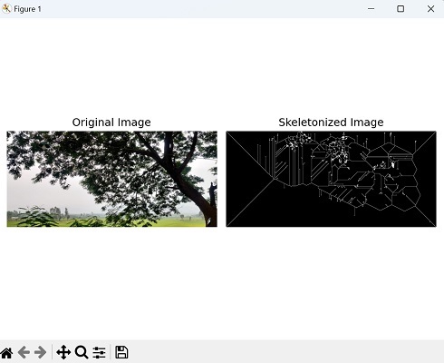
使用細化計算離心率

細化，也稱為細化，是一個旨在減少物體形狀或結構的過程，將其表示為細長的骨架。我們可以使用Mahotas中的thin()函式來實現這一點。

mahotas.thin()函式將二值影像作為輸入，其中感興趣的物體由白色畫素（畫素值為1）表示，背景由黑色畫素（畫素值為0）表示。

我們可以透過將影像簡化為其骨架表示來使用細化計算影像的離心率。

示例

現在，我們使用細化計算影像的離心率：

import mahotas as mh
import matplotlib.pyplot as plt
# Read the image and convert it to grayscale
image = mh.imread('tree.tiff')
grey_image = mh.colors.rgb2grey(image)
# Skeletonizing the image
skeleton = mh.thin(grey_image)
# Calculating the eccentricity of the skeletonized image
eccentricity = mh.features.eccentricity(skeleton)
# Printing the eccentricity
print(eccentricity)
# Create a figure with subplots
fig, axes = plt.subplots(1, 2, figsize=(7,5 ))
# Display the original image
axes[0].imshow(image)
axes[0].set_title('Original Image')
axes[0].axis('off')
# Display the skeletonized image
axes[1].imshow(skeleton, cmap='gray')
axes[1].set_title('Skeletonized Image')
axes[1].axis('off')
# Adjust the layout and display the plot
plt.tight_layout()
plt.show()

輸出

獲得的輸出如下所示：

0.8975030064719701

顯示的影像是如下所示：