- Mahotas 教程
- Mahotas - 首頁
- Mahotas - 簡介
- Mahotas - 計算機視覺
- Mahotas - 歷史
- Mahotas - 特性
- Mahotas - 安裝
- Mahotas 影像處理
- Mahotas - 影像處理
- Mahotas - 載入影像
- Mahotas - 載入灰度影像
- Mahotas - 顯示影像
- Mahotas - 顯示影像形狀
- Mahotas - 儲存影像
- Mahotas - 影像質心
- Mahotas - 影像卷積
- Mahotas - 建立RGB影像
- Mahotas - 影像尤拉數
- Mahotas - 影像中零的比例
- Mahotas - 獲取影像矩
- Mahotas - 影像區域性最大值
- Mahotas - 影像橢圓軸
- Mahotas - 影像拉伸RGB
- Mahotas 顏色空間轉換
- Mahotas - 顏色空間轉換
- Mahotas - RGB到灰度轉換
- Mahotas - RGB到LAB轉換
- Mahotas - RGB到褐色轉換
- Mahotas - RGB到XYZ轉換
- Mahotas - XYZ到LAB轉換
- Mahotas - XYZ到RGB轉換
- Mahotas - 增加伽馬校正
- Mahotas - 拉伸伽馬校正
- Mahotas 標記影像函式
- Mahotas - 標記影像函式
- Mahotas - 標記影像
- Mahotas - 過濾區域
- Mahotas - 邊界畫素
- Mahotas - 形態學運算
- Mahotas - 形態學運算元
- Mahotas - 查詢影像平均值
- Mahotas - 裁剪影像
- Mahotas - 影像離心率
- Mahotas - 影像疊加
- Mahotas - 影像圓度
- Mahotas - 調整影像大小
- Mahotas - 影像直方圖
- Mahotas - 膨脹影像
- Mahotas - 腐蝕影像
- Mahotas - 分水嶺演算法
- Mahotas - 影像開運算
- Mahotas - 影像閉運算
- Mahotas - 填充影像孔洞
- Mahotas - 條件膨脹影像
- Mahotas - 條件腐蝕影像
- Mahotas - 影像條件分水嶺演算法
- Mahotas - 影像區域性最小值
- Mahotas - 影像區域最大值
- Mahotas - 影像區域最小值
- Mahotas - 高階概念
- Mahotas - 影像閾值化
- Mahotas - 設定閾值
- Mahotas - 軟閾值
- Mahotas - Bernsen區域性閾值化
- Mahotas - 小波變換
- 製作影像小波中心
- Mahotas - 距離變換
- Mahotas - 多邊形工具
- Mahotas - 區域性二值模式
- 閾值鄰域統計
- Mahotas - Haralick特徵
- 標記區域的權重
- Mahotas - Zernike特徵
- Mahotas - Zernike矩
- Mahotas - 排序濾波器
- Mahotas - 二維拉普拉斯濾波器
- Mahotas - 多數濾波器
- Mahotas - 均值濾波器
- Mahotas - 中值濾波器
- Mahotas - Otsu方法
- Mahotas - 高斯濾波
- Mahotas - Hit & Miss變換
- Mahotas - 標記最大值陣列
- Mahotas - 影像平均值
- Mahotas - SURF密集點
- Mahotas - SURF積分影像
- Mahotas - Haar變換
- 突出影像最大值
- 計算線性二值模式
- 獲取標籤邊界
- 反轉Haar變換
- Riddler-Calvard方法
- 標記區域的大小
- Mahotas - 模板匹配
- 加速魯棒特徵
- 去除邊界標記
- Mahotas - Daubechies小波
- Mahotas - Sobel邊緣檢測
Mahotas - 影像卷積
影像處理中的卷積用於對影像執行各種濾波操作。
其中一些包括:
提取特徵 - 透過應用特定的濾波器來檢測邊緣、角點、斑點等特徵。
濾波 - 用於對影像執行平滑和銳化操作。
壓縮 - 可以透過去除影像中的冗餘資訊來壓縮影像。
Mahotas中的影像卷積
在Mahotas中,可以使用`convolve()`函式對影像進行卷積。此函式接受兩個引數:輸入影像和卷積核;其中,卷積核是一個小的矩陣,定義了卷積過程中要應用的操作,例如模糊、銳化、邊緣檢測或任何其他所需的效果。
使用`convolve()`函式
`convolve()`函式用於對影像執行卷積。卷積是一個數學運算,它接受兩個陣列——影像和卷積核,併產生第三個陣列(輸出影像)。
卷積核是一個小的數字陣列,用於濾波影像。卷積運算透過將影像和卷積核的對應元素相乘,然後將結果相加來執行。卷積運算的輸出是一幅已被卷積核濾波的新影像。
在Mahotas中執行卷積的語法如下:
convolve(image, kernel, mode='reflect', cval=0.0, out=None)
其中,
image - 輸入影像。
kernel - 卷積核。
mode - 指定如何處理影像邊緣。可以是reflect、nearest、constant、ignore、wrap或mirror。預設選擇reflect。
cval - 指定用於影像外部畫素的值。
out - 指定輸出影像。如果未指定out引數,則將建立一個新影像。
示例
在下面的示例中,我們首先使用`mh.imresize()`函式將輸入影像'nature.jpeg'調整為'4×4'的形狀。然後,我們建立一個所有值都設定為1的'4×4'卷積核。最後,我們使用`mh.convolve()`函式執行卷積:
import mahotas as mh
import numpy as np
# Load the image
image = mh.imread('nature.jpeg', as_grey=True)
# Resize the image to 4x4
image = mh.imresize(image, (4, 4))
# Create a 4x4 kernel
kernel = np.ones((4, 4))
# Perform convolution
result = mh.convolve(image, kernel)
print (result)
輸出
以下是上述程式碼的輸出:
[[3155.28 3152.84 2383.42 1614. ]
[2695.96 2783.18 2088.38 1393.58]
[1888.48 1970.62 1469.53 968.44]
[1081. 1158.06 850.68 543.3 ]]
使用高斯核進行卷積
在Mahotas中,高斯核是一個小的數字矩陣,用於模糊或平滑影像。
高斯核對每個畫素應用加權平均值,其中權重由稱為高斯分佈的鐘形曲線決定。該核對附近的畫素賦予更高的權重,對較遠的畫素賦予較低的權重。此過程有助於減少噪聲並增強影像中的特徵,從而產生更平滑、更賞心悅目的輸出。
以下是Mahotas中高斯核的基本語法:
mahotas.gaussian_filter(array, sigma)
其中,
array - 輸入陣列。
sigma - 高斯核的標準差。
示例
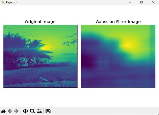
以下是使用高斯濾波器對影像進行卷積的示例。在這裡,我們正在調整影像大小,將其轉換為灰度影像,應用高斯濾波器來模糊影像,然後並排顯示原始影像和模糊影像:
import mahotas as mh
import matplotlib.pyplot as mtplt
# Load the image
image = mh.imread('sun.png')
# Convert to grayscale if needed
if len(image.shape) > 2:
   image = mh.colors.rgb2gray(image)
# Resize the image to 128x128
image = mh.imresize(image, (128, 128))
# Create the Gaussian kernel
kernel = mh.gaussian_filter(image, 1.0)
# Reduce the size of the kernel to 20x20
kernel = kernel[:20, :20]
# Blur the image
blurred_image = mh.convolve(image, kernel)
# Creating a figure and subplots
fig, axes = mtplt.subplots(1, 2)
# Displaying original image
axes[0].imshow(image)
axes[0].axis('off')
axes[0].set_title('Original Image')
# Displaying blurred image
axes[1].imshow(blurred_image)
axes[1].axis('off')
axes[1].set_title('Gaussian Filter Image')
# Adjusting the spacing and layout
mtplt.tight_layout()
# Showing the figure
mtplt.show()
輸出
上述程式碼的輸出如下:
帶填充的卷積
Mahotas中的帶填充的卷積是指在執行卷積運算之前,在影像邊緣周圍新增額外的畫素或邊界。填充的目的是建立一個尺寸更大的新影像,而不會丟失原始影像邊緣的資訊。
填充確保可以將卷積核應用於所有畫素,包括邊緣處的畫素,從而產生與原始影像大小相同的卷積輸出。
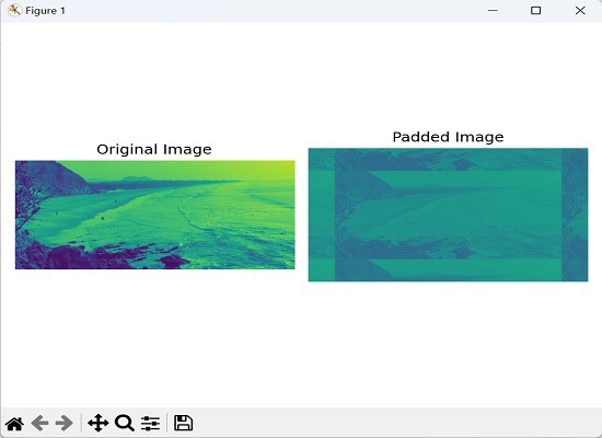
示例
在這裡,我們定義了一個自定義卷積核作為NumPy陣列,以強調影像的邊緣:
import numpy as np
import mahotas as mh
import matplotlib.pyplot as mtplt
# Create a custom kernel
kernel = np.array([[0, -1, 0],[-1, 5, -1],
[0, -1, 0]])
# Load the image
image = mh.imread('sea.bmp', as_grey=True)
# Add padding to the image
padding = np.pad(image, 150, mode='wrap')
# Perform convolution with padding
padded_image = mh.convolve(padding, kernel)
# Creating a figure and subplots
fig, axes = mtplt.subplots(1, 2)
# Displaying original image
axes[0].imshow(image)
axes[0].axis('off')
axes[0].set_title('Original Image')
# Displaying padded image
axes[1].imshow(padded_image)
axes[1].axis('off')
axes[1].set_title('Padded Image')
# Adjusting the spacing and layout
mtplt.tight_layout()
# Showing the figure
mtplt.show()
輸出
執行上述程式碼後,我們將得到以下輸出:
使用盒式濾波器進行模糊處理的卷積
Mahotas中使用盒式濾波器進行卷積是一種可用於模糊影像的技術。盒式濾波器是一個簡單的濾波器,其中濾波器核中的每個元素都具有相同的值,從而產生均勻的權重分佈。
使用盒式濾波器進行卷積包括將核滑過影像並取核覆蓋區域內畫素值的平均值。然後,使用該平均值替換輸出影像中的中心畫素值。
對影像中的所有畫素重複此過程,從而產生原始影像的模糊版本。模糊的程度由核的大小決定,較大的核產生更大的模糊。
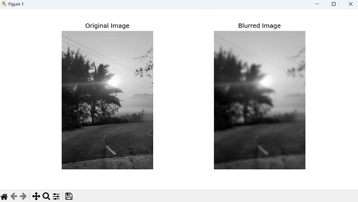
示例
以下是使用盒式濾波器進行卷積以模糊影像的示例:
import mahotas as mh
import numpy as np
import matplotlib.pyplot as plt
# Load the image
image = mh.imread('sun.png', as_grey=True)
# Define the size of the box filter
box_size = 25
# Create the box filter
box_filter = np.ones((box_size, box_size)) / (box_size * box_size)
# Perform convolution with the box filter
blurred_image = mh.convolve(image, box_filter)
# Display the original and blurred images
fig, axes = plt.subplots(1, 2, figsize=(10, 5))
axes[0].imshow(image, cmap='gray')
axes[0].set_title('Original Image')
axes[0].axis('off')
axes[1].imshow(blurred_image, cmap='gray')
axes[1].set_title('Blurred Image')
axes[1].axis('off')
plt.show()
輸出
我們將得到如下所示的輸出:
使用Sobel濾波器進行邊緣檢測的卷積
Sobel濾波器通常用於邊緣檢測。它由兩個單獨的濾波器組成:一個用於檢測水平邊緣,另一個用於檢測垂直邊緣。
透過將Sobel濾波器與影像進行卷積,我們得到一幅新的影像,其中邊緣被突出顯示,影像的其餘部分顯得模糊。與周圍區域相比,突出顯示的邊緣通常具有更高的強度值。
示例
在這裡,我們透過將Sobel濾波器與灰度影像進行卷積來執行邊緣檢測。然後,我們計算邊緣的幅度並應用閾值以獲得檢測到的邊緣的二值影像:
import mahotas as mh
import numpy as np
import matplotlib.pyplot as plt
image = mh.imread('nature.jpeg', as_grey=True)
# Apply Sobel filter for horizontal edges
sobel_horizontal = np.array([[1, 2, 1],
[0, 0, 0],[-1, -2, -1]])
# convolving the image with the filter kernels
edges_horizontal = mh.convolve(image, sobel_horizontal)
# Apply Sobel filter for vertical edges
sobel_vertical = np.array([[1, 0, -1],[2, 0, -2],[1, 0, -1]])
# convolving the image with the filter kernels
edges_vertical = mh.convolve(image, sobel_vertical)
# Compute the magnitude of the edges
edges_magnitude = np.sqrt(edges_horizontal**2 + edges_vertical**2)
# Threshold the edges
threshold = 50
thresholded_edges = edges_magnitude > threshold
# Display the original image and the detected edges
fig, axes = plt.subplots(1, 3, figsize=(12, 4))
axes[0].imshow(image, cmap='gray')
axes[0].set_title('Original Image')
axes[0].axis('off')
axes[1].imshow(edges_magnitude, cmap='gray')
axes[1].set_title('Edges Magnitude')
axes[1].axis('off')
axes[2].imshow(thresholded_edges, cmap='gray')
axes[2].set_title('Thresholded Edges')
axes[2].axis('off')
plt.tight_layout()
plt.show()
輸出
獲得的輸出如下:
