Mahotas - 均值濾波器

均值濾波器用於平滑影像以減少噪聲。它的工作原理是計算指定鄰域內所有畫素的平均值，然後用平均值替換原始畫素的值。

假設我們有一個具有不同強度值的灰度影像。因此，某些畫素可能具有比其他畫素更高的強度值。

因此，均值濾波器用於透過稍微模糊影像來建立畫素的均勻外觀。

Mahotas 中的均值濾波器

要在 mahotas 中應用均值濾波器，我們可以使用 **mean_filter()** 函式。

Mahotas 中的均值濾波器使用結構元素來檢查鄰域中的畫素。

結構元素將每個畫素值替換為其相鄰畫素的平均值。

結構元素的大小決定了平滑的程度。更大的鄰域會導致更強的平滑效果，同時會減少一些更精細的細節，而較小的鄰域會導致平滑效果較弱，但會保留更多細節。

mahotas.mean_filter() 函式

mean_filter() 函式使用指定的鄰域大小將均值濾波器應用於輸入影像。

它用其鄰居中的多數值替換每個畫素值。濾波後的影像儲存在輸出陣列中。

語法

以下是 mahotas 中 mean filter() 函式的基本語法：

mahotas.mean_filter(f, Bc, mode='ignore', cval=0.0, out=None)

其中，

**img** - 輸入影像。
**Bc** - 定義鄰域的結構元素。
**mode（可選）** - 指定函式如何處理影像的邊界。它可以取不同的值，例如“reflect”、“constant”、“nearest”、“mirror”或“wrap”。
預設情況下，它設定為“ignore”，這意味著濾波器會忽略影像邊界之外的畫素。
**cval（可選）** - 當 mode='constant' 時要使用的值。預設值為 0.0。
**out（可選）** - 指定將儲存濾波後圖像的輸出陣列。它必須與輸入影像具有相同的形狀。

示例

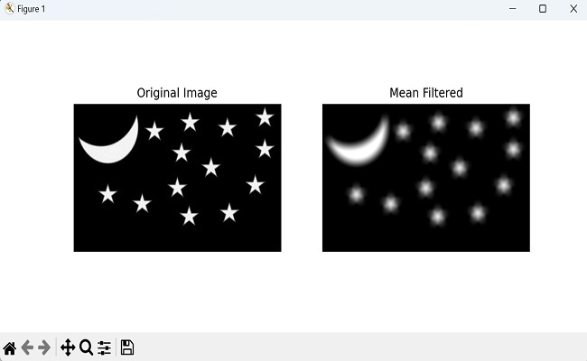
以下是使用 mean_filter() 函式濾波影像的基本示例：

import mahotas as mh
import numpy as np
import matplotlib.pyplot as mtplt
image=mh.imread('tree.tiff', as_grey = True)
structuring_element = mh.disk(12)
filtered_image = mh.mean_filter(image, structuring_element)
# Displaying the original image
fig, axes = mtplt.subplots(1, 2, figsize=(9, 4))
axes[0].imshow(image, cmap='gray')
axes[0].set_title('Original Image')
axes[0].axis('off')
# Displaying the mean filtered image
axes[1].imshow(filtered_image, cmap='gray')
axes[1].set_title('Mean Filtered')
axes[1].axis('off')
mtplt.show()

輸出

執行上述程式碼後，我們將得到以下輸出：

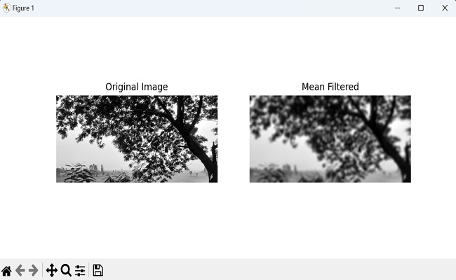
使用反射模式的均值濾波器

當我們將均值濾波器應用於影像時，我們需要考慮每個畫素周圍的相鄰畫素來計算平均值。但是，在影像的邊緣，有一些畫素在一側或多側沒有鄰居。

為了解決這個問題，我們使用 **'reflect'** 模式。反射模式沿著影像邊緣建立映象效果。它允許我們透過映象方式複製其畫素來虛擬地擴充套件影像。

這樣，我們即使在邊緣也可以為均值濾波器提供相鄰畫素。

透過反射影像值，均值濾波器現在可以將這些映象畫素視為真實的鄰居。

它使用這些虛擬鄰居計算平均值，從而在影像邊緣產生更準確的平滑過程。

示例

在這裡，我們嘗試使用反射模式計算均值濾波器：

import mahotas as mh
import numpy as np
import matplotlib.pyplot as mtplt
image=mh.imread('nature.jpeg', as_grey = True)
structuring_element = mh.morph.dilate(mh.disk(12), Bc=mh.disk(12))
filtered_image = mh.mean_filter(image, structuring_element, mode='reflect')
# Displaying the original image
fig, axes = mtplt.subplots(1, 2, figsize=(9, 4))
axes[0].imshow(image, cmap='gray')
axes[0].set_title('Original Image')
axes[0].axis('off')
# Displaying the mean filtered image
axes[1].imshow(filtered_image, cmap='gray')
axes[1].set_title('Mean Filtered')
axes[1].axis('off')
mtplt.show()

輸出

上述程式碼的輸出如下：

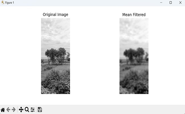
透過將結果儲存在輸出陣列中

我們也可以使用 Mahotas 將均值濾波器的結果儲存在輸出陣列中。為此，我們首先需要使用 NumPy 庫建立一個空陣列。

此陣列初始化為與輸入影像相同的形狀，以儲存生成的濾波影像。陣列的資料型別指定為 float（預設值）。

最後，我們透過將其作為引數傳遞給 mean_filter() 函式，將生成的濾波影像儲存在輸出陣列中。

示例

現在，我們嘗試將均值濾波器應用於灰度影像並將結果儲存在特定的輸出陣列中：

import mahotas as mh
import numpy as np
import matplotlib.pyplot as mtplt
image=mh.imread('pic.jpg', as_grey = True)
# Create an output array for the filtered image
output = np.empty(image.shape)
# store the result in the output array
mh.mean_filter(image, Bc=mh.disk(12), out=output)
# Displaying the original image
fig, axes = mtplt.subplots(1, 2, figsize=(9, 4))
axes[0].imshow(image, cmap='gray')
axes[0].set_title('Original Image')
axes[0].axis('off')
# Displaying the mean filtered image
axes[1].imshow(output, cmap='gray')
axes[1].set_title('Mean Filtered')
axes[1].axis('off')
mtplt.show()

輸出

以下是上述程式碼的輸出：

列印頁面