Mahotas - SURF密集點

SURF（加速魯棒特徵）是一種用於檢測和描述影像中興趣點的演算法。這些點被稱為“密集點”或“關鍵點”，因為它們密集地分佈在整個影像中，不像稀疏點只出現在特定區域。

SURF演算法以不同的尺度分析整個影像，並識別強度變化顯著的區域。

這些區域被認為是潛在的關鍵點。它們是包含獨特且顯著模式的感興趣區域。

Mahotas中的SURF密集點

在Mahotas中，我們使用mahotas.features.surf.dense()函式來計算SURF密集點的描述符。描述符本質上是特徵向量，描述了影像中畫素的區域性特徵，例如它們的強度梯度和方向。

為了生成這些描述符，該函式在影像上建立一個點網格，每個點之間保持一定的距離。在網格中的每個點上，都會確定一個“興趣點”。

這些興趣點是捕獲影像詳細資訊的位置。一旦識別出興趣點，就會計算密集的SURF描述符。

mahotas.features.surf.dense()函式

mahotas.features.surf.dense()函式以灰度影像作為輸入，並返回一個包含描述符的陣列。

這個陣列通常具有這樣的結構：每一行對應一個不同的興趣點，列代表該點的描述符特徵值。

語法

以下是Mahotas中surf.dense()函式的基本語法：

mahotas.features.surf.dense(f, spacing, scale={np.sqrt(spacing)},
is_integral=False, include_interest_point=False)

其中，

f - 輸入灰度影像。
spacing - 確定相鄰關鍵點之間的距離。
scale（可選） - 指定計算描述符時使用的間距（預設為間距的平方根）。
is_integral（可選） - 一個標誌，指示輸入影像是整數還是浮點數（預設為'False'）。
include_interest_point（可選） - 一個標誌，指示是否與SURF點一起返回興趣點（預設為'False'）。

示例

在下面的示例中，我們使用mh.features.surf.dense()函式計算影像的SURF密集點。

import mahotas as mh
from mahotas.features import surf
import numpy as np
import matplotlib.pyplot as mtplt
# Loading the image
image = mh.imread('sun.png')
# Converting it to grayscale
image = mh.colors.rgb2gray(image)
# Getting the SURF dense points
surf_dense = surf.dense(image, 120)
# Creating a figure and axes for subplots
fig, axes = mtplt.subplots(1, 2)
# Displaying the original image
axes[0].imshow(image)
axes[0].set_title('Original Image')
axes[0].set_axis_off()
# Displaying the surf dense points
axes[1].imshow(surf_dense)
axes[1].set_title('SURF Dense Point')
axes[1].set_axis_off()
# Adjusting spacing between subplots
mtplt.tight_layout()
# Showing the figures
mtplt.show()

輸出

以下是上述程式碼的輸出：

透過調整尺度

我們可以調整尺度來計算不同空間中SURF密集點的描述符。尺度決定了圍繞興趣點檢查的區域大小。

較小的尺度適用於捕獲區域性細節，而較大的尺度適用於捕獲全域性細節。

在Mahotas中，surf.dense()函式的scale引數決定了計算SURF密集點描述符時使用的縮放比例。

我們可以為此引數傳遞任何值來檢查縮放對SURF密集點的影響。

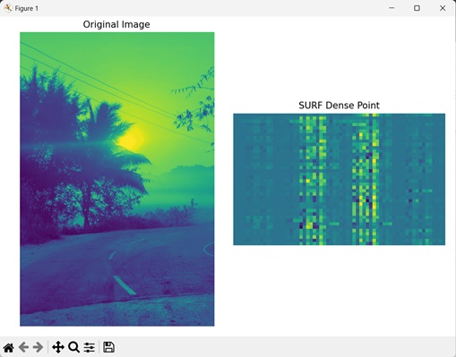
示例

在下面提到的示例中，我們正在調整尺度以計算SURF密集點的描述符：

import mahotas as mh
from mahotas.features import surf
import numpy as np
import matplotlib.pyplot as mtplt
# Loading the image
image = mh.imread('nature.jpeg')
# Converting it to grayscale
image = mh.colors.rgb2gray(image)
# Getting the SURF dense points
surf_dense = surf.dense(image, 100, np.sqrt(25))
# Creating a figure and axes for subplots
fig, axes = mtplt.subplots(1, 2)
# Displaying the original image
axes[0].imshow(image)
axes[0].set_title('Original Image')
axes[0].set_axis_off()
# Displaying the surf dense points
axes[1].imshow(surf_dense)
axes[1].set_title('SURF Dense Point')
axes[1].set_axis_off()
# Adjusting spacing between subplots
mtplt.tight_layout()
# Showing the figures
mtplt.show()

輸出

上述程式碼的輸出如下：

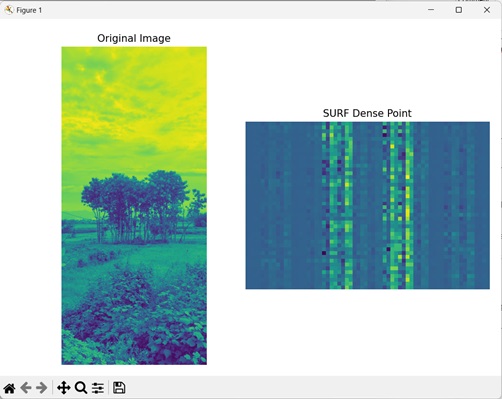
透過包含興趣點

在計算SURF密集點的描述符時，我們也可以包含影像的興趣點。興趣點是畫素強度值發生顯著變化的區域。

在Mahotas中，為了包含影像的興趣點，在計算SURF密集點的描述符時，我們可以將include_interest_point引數設定為布林值'True'。

示例

在這裡，我們在計算影像SURF密集點的描述符時包含了興趣點。

import mahotas as mh
from mahotas.features import surf
import numpy as np
import matplotlib.pyplot as mtplt
# Loading the image
image = mh.imread('tree.tiff')
# Converting it to grayscale
image = mh.colors.rgb2gray(image)
# Getting the SURF dense points
surf_dense = surf.dense(image, 100, include_interest_point=True)
# Creating a figure and axes for subplots
fig, axes = mtplt.subplots(1, 2)
# Displaying the original image
axes[0].imshow(image)
axes[0].set_title('Original Image')
axes[0].set_axis_off()
# Displaying the surf dense points
axes[1].imshow(surf_dense)
axes[1].set_title('SURF Dense Point')
axes[1].set_axis_off()
# Adjusting spacing between subplots
mtplt.tight_layout()
# Showing the figures
mtplt.show()

輸出

執行上述程式碼後，我們將獲得以下輸出：

列印頁面