Mahotas - 排序濾波器

---

---

排序濾波器是一種用於修改影像的技術，它透過根據畫素的相對排名（位置）來改變畫素值。它關注畫素值本身，而不是它們的實際強度。

對於影像中的每個畫素，排序濾波器會檢查其鄰域內所有畫素的值，並按升序或降序排列。

然後，它根據其位置或排名從排序列表中選擇特定的畫素值。

例如，如果排序濾波器設定為選擇中值，它將從排序列表中選擇中間的畫素值。

如果它設定為選擇最小值或最大值，它將分別選擇第一個或最後一個值。

Mahotas 中的排序濾波器

我們可以使用 mahotas.rank_filter() 函式在 mahotas 中執行排序濾波器。Mahotas 中的排序濾波器比較鄰域內的畫素強度值，並根據其在排序強度列表中的排名為每個畫素分配一個新值。

為了詳細說明，讓我們看看排序濾波器在 mahotas 中是如何工作的：

• 假設您有一個由許多畫素組成的灰度影像，每個畫素都具有一定的強度值，範圍從黑色到白色。

• 現在，讓我們關注影像中的一個特定畫素。排序濾波器將檢查該畫素周圍的鄰域。

• 在這個鄰域內，排序濾波器將比較所有畫素的強度值。它將根據畫素的強度值按升序或降序排列這些畫素，具體取決於濾波器的配置。

• 一旦強度值被排序，排序濾波器將根據其在排序列表中的排名為中心畫素分配一個新值。這個新值通常是鄰域內的中值、最小值或最大強度值。

透過對影像中的每個畫素重複此過程，排序濾波器可以幫助完成各種影像增強任務。

mahotas.rank_filter() 函式

mahotas 中的 rank_filter() 函式接受三個引數：要過濾的影像、結構元素和鄰域的大小。

鄰域是每個畫素周圍的矩形區域，其大小由每個維度中的畫素數指定。例如，大小為 3×3 的鄰域將包含畫素的八個鄰居。

rank_filter() 函式返回一個與原始影像具有相同維度的新影像。新影像中的值是原始影像中相應畫素的排名。

語法

以下是 mahotas 中 rank_filter() 函式的基本語法：

mahotas.rank_filter(f, Bc, rank, mode='reflect', cval=0.0, out=None)

其中，

• f − 它是要應用排序濾波器的輸入影像陣列。

• Bc − 定義每個畫素周圍鄰域的結構元素。

• rank − 它確定要從鄰域內排序列表中選擇的畫素值的排名。如果需要多個排名，則排名可以是整數或整數列表。

• mode（可選） − 確定如何處理輸入影像的邊界。它可以取以下值之一：“ignore”，“constant”，“nearest”，“mirror”或“wrap”。預設值為“reflect”。

• cval（可選） − 當 mode='constant' 時使用的值。預設值為 0.0。

• out（可選） − 用於儲存排序濾波器輸出的陣列。如果未提供，則會建立一個新陣列。

示例

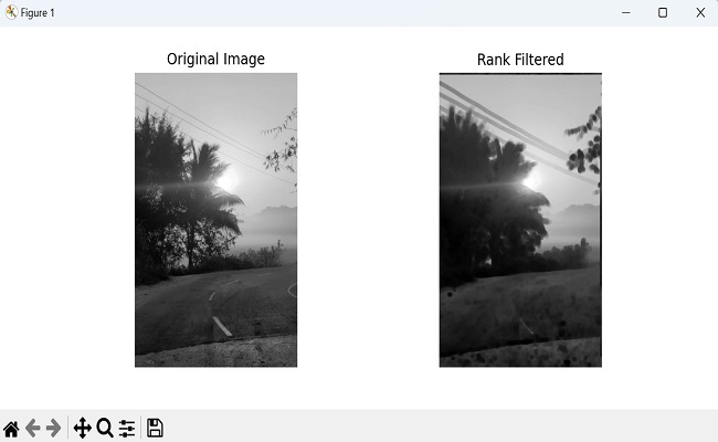
以下是使用 rank_filter() 函式過濾影像的基本示例：

import mahotas as mh
import numpy as np
import matplotlib.pyplot as mtplt
# Creating a sample grayscale image
image = mh.imread('nature.jpeg', as_grey = True)
# Applying minimum filter
filtered_image = mh.rank_filter(image, mh.disk(6), rank=0)
print(filtered_image)
# Displaying the original image
fig, axes = mtplt.subplots(1, 2, figsize=(9, 4))
axes[0].imshow(image, cmap='gray')
axes[0].set_title('Original Image')
axes[0].axis('off')
# Displaying the rank filtered featured image
axes[1].imshow(filtered_image, cmap='gray')
axes[1].set_title('Rank Filtered')
axes[1].axis('off')
mtplt.show()

輸出

執行上述程式碼後，我們將得到以下輸出：

[[193.71 193.71 193.71 ... 206.17 206.17 207.17]
 [193.71 193.71 193.71 ... 206.17 206.17 207.17]
 [193.71 193.71 193.71 ... 206.17 206.17 207.17]
 ...
 [ 74.59  62.44 53.62 ... 4.85 4.85 4.85]
 [ 85.37  74.59 62.44 ... 4.85 4.85 4.85]
 [ 90.05  79.3 73.18 ...  4.85 4.85 4.85]]

顯示的影像如下所示：

RGB 影像上的排序濾波器

彩色影像由三個顏色通道組成：紅色、綠色和藍色（RGB）。透過分別對每個通道應用排序濾波器，我們可以增強每個顏色通道的特定特徵。

要在 mahotas 中對 RGB 影像應用排序濾波器，我們首先透過指定通道值從 RGB 影像中提取通道。

通道值分別使用索引 0、1 和 2 來訪問紅色、綠色和藍色通道。然後，我們對每個通道應用排序濾波器，並將它們堆疊在一起以重建最終的 RGB 影像。

示例

在這裡，我們分別對 RGB 影像的每個通道應用具有不同鄰域大小的中值濾波器：

import mahotas as mh
import numpy as np
import matplotlib.pyplot as mtplt
image = mh.imread('nature.jpeg')
# Applying a median filter with different neighborhood sizes on each channel
separately
filtered_image = np.stack([mh.rank_filter(image[:, :, 0], mh.disk(2), rank=4),
mh.rank_filter(image[:, :, 1], mh.disk(1), rank=4),
mh.rank_filter(image[:, :, 2], mh.disk(3), rank=4)],
axis=2)
# Displaying the original image
fig, axes = mtplt.subplots(1, 2, figsize=(9, 4))
axes[0].imshow(image, cmap='gray')
axes[0].set_title('Original Image')
axes[0].axis('off')
# Displaying the rank filtered featured image
axes[1].imshow(filtered_image, cmap='gray')
axes[1].set_title('Rank Filtered')
axes[1].axis('off')
mtplt.show()

輸出

以下是上述程式碼的輸出：

使用“Wrap”模式

在對影像執行排序濾波時，邊緣或邊界處的畫素通常缺乏足夠的相鄰畫素來準確計算排名。

為了解決此問題，Mahotas 中的“wrap”模式將影像值環繞到另一側。這意味著影像一端畫素的值被視為另一端畫素的鄰居。

這在兩側之間建立了一個無縫過渡，確保在計算排名值時考慮邊界處的畫素。

示例

import mahotas as mh
import numpy as np
import matplotlib.pyplot as mtplt
image = mh.imread('sun.png', as_grey = True)
# Applying maximum filter with 'wrap' mode
filtered_image = mh.rank_filter(image, mh.disk(10), rank=8, mode='wrap')
print(filtered_image)
# Displaying the original image
fig, axes = mtplt.subplots(1, 2, figsize=(9, 4))
axes[0].imshow(image, cmap='gray')
axes[0].set_title('Original Image')
axes[0].axis('off')
# Displaying the rank filtered featured image
axes[1].imshow(filtered_image, cmap='gray')
axes[1].set_title('Rank Filtered')
axes[1].axis('off')
mtplt.show()

輸出

上述程式碼的輸出如下：

[[49.92 49.92 49.92 ... 49.92 49.92 49.92]
 [49.92 49.92 49.92 ... 49.92 49.92 49.92]
 [49.92 49.92 49.92 ... 49.92 49.92 49.92]
 ...
 [49.92 49.92 49.92 ... 49.92 49.92 49.92]
 [49.92 49.92 49.92 ... 49.92 49.92 49.92]
 [49.92 49.92 49.92 ... 49.92 49.92 49.92]]

獲得的影像如下所示：