Mahotas - 影像小波中心化

---

---

影像小波中心化是指將影像的小波係數移動到小波中心，小波中心是小波達到最大幅度的點。小波係數是表示不同頻率對影像貢獻的數值。

透過使用小波變換將影像分解成單個波來獲得小波係數。透過對係數進行中心化，可以將低頻和高頻與中心頻率對齊，從而去除影像中的噪聲。

在 Mahotas 中進行影像小波中心化

在 Mahotas 中，我們可以使用 **mahotas.wavelet_center()** 函式對影像進行小波中心化以減少噪聲。該函式執行兩個主要步驟來進行影像小波中心化，如下所示：

• 首先，它將原始影像的訊號分解成小波係數。

• 接下來，它獲取近似係數（即低頻係數），並將它們與中心頻率對齊。

透過對齊頻率，消除了影像的平均強度，從而去除了噪聲。

mahotas.wavelet_center() 函式

mahotas.wavelet_center() 函式以影像作為輸入，並返回一個新的影像，其中小波中心位於原點。

它使用小波變換分解（拆分）原始輸入影像，然後將小波係數移動到頻譜中心。

在查詢影像小波中心時，該函式會忽略指定畫素大小的邊界區域。

語法

以下是 mahotas 中 wavelet_center() 函式的基本語法：

mahotas.wavelet_center(f, border=0, dtype=float, cval=0.0)

其中，

• **f** - 輸入影像。

• **border (可選)** - 邊界區域的大小（預設為 0 或無邊界）。

• **dtype (可選)** - 返回影像的資料型別（預設為 float）。

• **cval (可選)** - 用於填充邊界區域的值（預設為 0）。

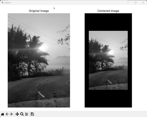
示例

在以下示例中，我們使用 mh.wavelet_center() 函式對影像進行小波中心化。

import mahotas as mh
import numpy as np
import matplotlib.pyplot as mtplt
# Loading the image
image = mh.imread('sun.png')
# Converting it to grayscale
image = mh.colors.rgb2gray(image)
# Centering the image
centered_image = mh.wavelet_center(image)
# Creating a figure and axes for subplots
fig, axes = mtplt.subplots(1, 2)
# Displaying the original image
axes[0].imshow(image, cmap='gray')
axes[0].set_title('Original Image')
axes[0].set_axis_off()
# Displaying the centered image
axes[1].imshow(centered_image, cmap='gray')
axes[1].set_title('Centered Image')
axes[1].set_axis_off()
# Adjusting spacing between subplots
mtplt.tight_layout()
# Showing the figures
mtplt.show()

輸出

以下是上述程式碼的輸出：

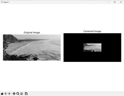
使用邊界進行中心化

我們可以使用邊界對影像進行小波中心化以操作輸出影像。邊界區域是指影像中圍繞物件的區域。它將物件與背景區域或相鄰物件隔開。

在 mahotas 中，我們可以透過將畫素值設定為零來定義在進行小波中心化時不應考慮的區域。這是透過將值傳遞給 mahotas.wavelet_center() 函式的 **border** 引數來完成的。

在進行影像小波中心化時，該函式會忽略引數中指定數量的畫素。例如，如果 border 引數設定為 500，則在中心化影像小波時，所有側面的 500 個畫素將被忽略。

示例

在下面提到的示例中，我們在中心化影像小波時忽略了一定大小的邊界。

import mahotas as mh
import numpy as np
import matplotlib.pyplot as mtplt
# Loading the image
image = mh.imread('sea.bmp')
# Converting it to grayscale
image = mh.colors.rgb2gray(image)
# Centering the image with border
centered_image = mh.wavelet_center(image, border=500)
# Creating a figure and axes for subplots
fig, axes = mtplt.subplots(1, 2)
# Displaying the original image
axes[0].imshow(image, cmap='gray')
axes[0].set_title('Original Image')
axes[0].set_axis_off()
# Displaying the centered image
axes[1].imshow(centered_image, cmap='gray')
axes[1].set_title('Centered Image')
axes[1].set_axis_off()
# Adjusting spacing between subplots
mtplt.tight_layout()
# Showing the figures
mtplt.show()

輸出

上述程式碼的輸出如下：

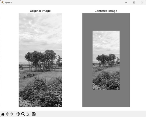
透過應用填充進行中心化

我們還可以透過應用填充來填充邊界區域以某種灰度來進行中心化。

填充是指在影像邊緣周圍新增額外的畫素值以建立邊界的技術。

在 mahotas 中，可以透過為 mahotas.wavelet_center() 函式的 **cval** 引數指定一個值來應用填充。它允許我們用一種顏色填充邊界區域，其值範圍從 0（黑色）到 255（白色）。

**注意** - 只有在存在邊界區域時才能應用填充。因此，border 引數的值不應為 0。

示例

在這裡，我們忽略了一定畫素大小的邊界並應用填充來中心化影像小波。

import mahotas as mh
import numpy as np
import matplotlib.pyplot as mtplt
# Loading the image
image = mh.imread('nature.jpeg')
# Converting it to grayscale
image = mh.colors.rgb2gray(image)
# Centering the image with border
centered_image = mh.wavelet_center(image, border=100, cval=109)
# Creating a figure and axes for subplots
fig, axes = mtplt.subplots(1, 2)
# Displaying the original image
axes[0].imshow(image, cmap='gray')
axes[0].set_title('Original Image')
axes[0].set_axis_off()
# Displaying the centered image
axes[1].imshow(centered_image, cmap='gray')
axes[1].set_title('Centered Image')
axes[1].set_axis_off()
# Adjusting spacing between subplots
mtplt.tight_layout()
# Showing the figures
mtplt.show()

輸出

執行上述程式碼後，我們將得到以下輸出：