Mahotas - 模板匹配

---

---

模板匹配是一種用於在較大影像中定位特定影像（模板）的技術。簡單來說，目標是在較大的影像中找到與較小影像匹配的位置。

模板匹配涉及將模板影像與較大影像的不同區域進行比較。在比較過程中，模板影像的不同屬性，例如大小、形狀、顏色和強度值，都會與較大影像進行匹配。

比較會持續進行，直到找到模板影像與較大影像之間最佳匹配的區域。

Mahotas中的模板匹配

在 Mahotas 中，我們可以使用 **mahotas.template_match()** 函式執行模板匹配。該函式將模板影像與較大影像中所有與模板影像大小相同的區域進行比較。

該函式使用平方差之和 (SSD) 方法執行模板匹配。SSD 方法的工作方式如下：

• 第一步是計算模板影像和較大影像的畫素值之間的差異。

• 下一步是將差異平方。

• 最後，將較大影像中所有畫素的平方差相加。

最終的 SSD 值決定了模板影像和較大影像之間的相似性。值越小，模板影像和較大影像之間的匹配度越高。

mahotas.template_match() 函式

mahotas.template_match() 函式接受影像和模板影像作為輸入。

它返回較大影像中與輸入模板影像最佳匹配的區域。

最佳匹配是 SSD 值最低的區域。

語法

以下是 Mahotas 中 template_match() 函式的基本語法：

mahotas.template_match(f, template, mode='reflect', cval=0.0, out=None)

其中：

• **f** - 輸入影像。

• **template** - 將與輸入影像匹配的模式。

• **mode (可選)** - 確定在模板應用於其邊界附近時如何擴充套件輸入影像（預設值為“reflect”）。

• **cval (可選)** - 當 mode 為“constant”時使用的填充常數值（預設為 0.0）。

• **out (可選)** - 定義儲存輸出影像的陣列（預設為 None）。

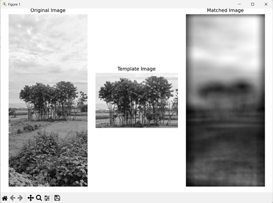
示例

在下面的示例中，我們使用 mh.template_match() 函式執行模板匹配。

import mahotas as mh
import numpy as np
import matplotlib.pyplot as mtplt
# Loading the images
image = mh.imread('tree.tiff', as_grey=True)
template = mh.imread('cropped tree.tiff', as_grey=True)
# Applying template matching algorithm
template_matching = mh.template_match(image, template)
# Creating a figure and axes for subplots
fig, axes = mtplt.subplots(1, 3)
# Displaying the original image
axes[0].imshow(image, cmap='gray')
axes[0].set_title('Original Image')
axes[0].set_axis_off()
# Displaying the template image
axes[1].imshow(template, cmap='gray')
axes[1].set_title('Template Image')
axes[1].set_axis_off()
# Displaying the matched image
axes[2].imshow(template_matching, cmap='gray')
axes[2].set_title('Matched Image')
axes[2].set_axis_off()
# Adjusting spacing between subplots
mtplt.tight_layout()
# Showing the figures
mtplt.show()

輸出

以下是上述程式碼的輸出：

透過包裹邊界進行匹配

在 Mahotas 中執行模板匹配時，我們可以包裹影像的邊界。包裹邊界是指將影像邊界摺疊到影像的另一側。

因此，邊界之外的畫素會在影像的另一側重複。

這有助於我們在模板匹配過程中處理影像邊界之外的畫素。

在 mahotas 中，我們可以透過將值“wrap”指定給 template_match() 函式的 **mode** 引數來包裹影像的邊界，從而執行模板匹配。

示例

在下面提到的示例中，我們透過包裹影像的邊界來執行模板匹配。

import mahotas as mh
import numpy as np
import matplotlib.pyplot as mtplt
# Loading the images
image = mh.imread('sun.png', as_grey=True)
template = mh.imread('cropped sun.png', as_grey=True)
# Applying template matching algorithm
template_matching = mh.template_match(image, template, mode='wrap')
# Creating a figure and axes for subplots
fig, axes = mtplt.subplots(1, 3)
# Displaying the original image
axes[0].imshow(image, cmap='gray')
axes[0].set_title('Original Image')
axes[0].set_axis_off()
# Displaying the template image
axes[1].imshow(template, cmap='gray')
axes[1].set_title('Template Image')
axes[1].set_axis_off()
# Displaying the matched image
axes[2].imshow(template_matching, cmap='gray')
axes[2].set_title('Matched Image')
axes[2].set_axis_off()
# Adjusting spacing between subplots
mtplt.tight_layout()
# Showing the figures
mtplt.show()

輸出

上述程式碼的輸出如下：

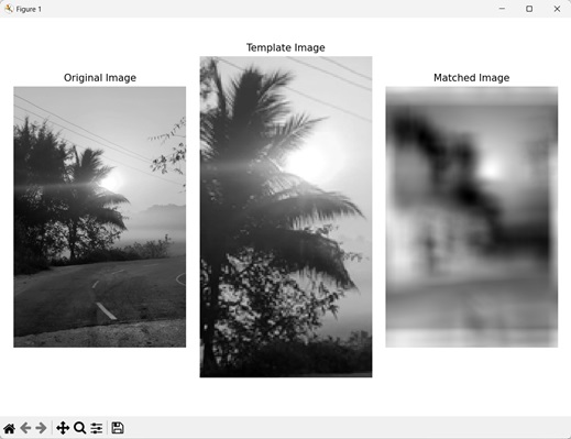
透過忽略邊界進行匹配

我們還可以透過忽略影像的邊界來執行模板匹配。在透過忽略邊界執行模板匹配時，超出影像邊界的畫素將被排除。

在 mahotas 中，我們透過將值“ignore”指定給 template_match() 函式的 **mode** 引數來忽略影像的邊界，從而執行模板匹配。

示例

在這裡，我們在執行模板匹配時忽略影像的邊界。

import mahotas as mh
import numpy as np
import matplotlib.pyplot as mtplt
# Loading the images
image = mh.imread('nature.jpeg', as_grey=True)
template = mh.imread('cropped nature.jpeg', as_grey=True)
# Applying template matching algorithm
template_matching = mh.template_match(image, template, mode='ignore')
# Creating a figure and axes for subplots
fig, axes = mtplt.subplots(1, 3)
# Displaying the original image
axes[0].imshow(image, cmap='gray')
axes[0].set_title('Original Image')
axes[0].set_axis_off()
# Displaying the template image
axes[1].imshow(template, cmap='gray')
axes[1].set_title('Template Image')
axes[1].set_axis_off()
# Displaying the matched image
axes[2].imshow(template_matching, cmap='gray')
axes[2].set_title('Matched Image')
axes[2].set_axis_off()
# Adjusting spacing between subplots
mtplt.tight_layout()
# Showing the figures
mtplt.show()

輸出

執行上述程式碼後，我們將得到以下輸出：