Mahotas - 影像標記

---

---

影像標記是指將類別（標籤）分配給影像的不同區域。標籤通常用整數值表示，每個值對應於特定類別或區域。

例如，讓我們考慮一個包含各種物體或區域的影像。每個區域都被分配一個唯一的值（整數）以將其與其他區域區分開來。背景區域的標籤值為 0。

在 Mahotas 中標記影像

在 Mahotas 中，我們可以使用 label() 或 labeled.label() 函式來標記影像。

這些函式透過為影像中不同的連通元件分配唯一的標籤或識別符號來將影像分割成不同的區域。每個連通元件是一組相鄰的畫素，它們共享一個共同的屬性，例如強度或顏色。

標記過程建立一個影像，其中屬於同一區域的畫素被分配相同的標籤值。

使用 mahotas.label() 函式

mahotas.label() 函式以影像作為輸入，其中感興趣的區域由前景（非零）值表示，背景由零表示。

該函式返回標記的陣列，其中每個連通元件或區域都被分配一個唯一的整數標籤。

label() 函式使用 8 連通性進行標記，這指的是影像中畫素之間的關係，其中每個畫素都與其周圍的八個鄰居（包括對角線）相連。

語法

以下是 mahotas 中 label() 函式的基本語法：

mahotas.label(array, Bc={3x3 cross}, output={new array})

其中：

• array - 輸入陣列。

• Bc (可選) - 用於連通性的結構元素。

• output (可選) - 輸出陣列（預設為與 array 形狀相同的新的陣列）。

示例

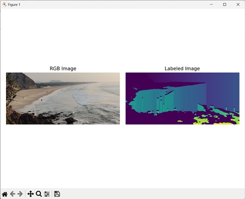
在下面的示例中，我們使用 mh.label() 函式來標記影像。

import mahotas as mh
import numpy as np
import matplotlib.pyplot as mtplt
# Loading the image
image_rgb = mh.imread('sun.png')
image = image_rgb[:,:,0]
# Applying gaussian filtering
image = mh.gaussian_filter(image, 4)
image = (image > image.mean())
# Converting it to a labeled image
labeled, num_objects = mh.label(image)
# Creating a figure and axes for subplots
fig, axes = mtplt.subplots(1, 2)
# Displaying the original RGB image
axes[0].imshow(image_rgb)
axes[0].set_title('RGB Image')
axes[0].set_axis_off()
# Displaying the labeled image
axes[1].imshow(labeled)
axes[1].set_title('Labeled Image')
axes[1].set_axis_off()
# Adjusting spacing between subplots
mtplt.tight_layout()
# Showing the figures
mtplt.show()

輸出

以下是上述程式碼的輸出：

使用 mahotas.labeled.label() 函式

mahotas.labeled.label() 函式為影像的不同區域分配從 1 開始的連續標籤。它與 mahotas.label() 函式類似，用於將影像分割成不同的區域。

如果你的標記影像具有非連續的標籤值，labeled.label() 函式會將標籤值更新為連續順序。

例如，假設我們有一個標記影像，其中四個區域的標籤分別為 2、4、7 和 9。labeled.label() 函式會將影像轉換為一個新的標記影像，其連續標籤分別為 1、2、3 和 4。

語法

以下是 mahotas 中 labeled.label() 函式的基本語法：

mahotas.labeled.label(array, Bc={3x3 cross}, output={new array})

其中：

• array - 輸入陣列。

• Bc (可選) - 用於連通性的結構元素。

• output (可選) - 輸出陣列（預設為與 array 形狀相同的新的陣列）。

示例

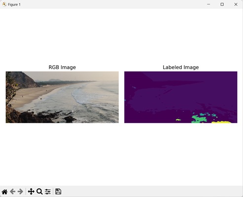
以下示例演示瞭如何使用 mh.labeled.label() 函式將影像轉換為標記影像。

import mahotas as mh
import numpy as np
import matplotlib.pyplot as mtplt
# Loading the image
image_rgb = mh.imread('sea.bmp')
image = image_rgb[:,:,0]
# Applying gaussian filtering
image = mh.gaussian_filter(image, 4)
image = (image > image.mean())
# Converting it to a labeled image
labeled, num_objects = mh.labeled.label(image)
# Creating a figure and axes for subplots
fig, axes = mtplt.subplots(1, 2)
# Displaying the original RGB image
axes[0].imshow(image_rgb)
axes[0].set_title('RGB Image')
axes[0].set_axis_off()
# Displaying the labeled image
axes[1].imshow(labeled)
axes[1].set_title('Labeled Image')
axes[1].set_axis_off()
# Adjusting spacing between subplots
mtplt.tight_layout()
# Showing the figures
mtplt.show()

輸出

以下是上述程式碼的輸出：

使用自定義結構元素

我們可以使用自定義結構元素和標籤函式根據需要分割影像。結構元素是一個奇數維的二元陣列，由 1 和 0 組成，它定義了影像標記過程中鄰域畫素的連線模式。

1 表示連線分析中包含的相鄰畫素，而 0 表示排除或忽略的鄰居。

例如，讓我們考慮自定義結構元素：[[1, 0, 0], [0, 1, 0], [0, 0, 1]]。 這個結構元素意味著對角線連線。這意味著對於影像中的每個畫素，在標記或分割過程中，只有對角線向上和向下畫素被認為是其鄰居。

示例

在這裡，我們定義了一個自定義結構元素來標記影像。

import mahotas as mh
import numpy as np
import matplotlib.pyplot as mtplt
# Loading the image
image_rgb = mh.imread('sea.bmp')
image = image_rgb[:,:,0]
# Applying gaussian filtering
image = mh.gaussian_filter(image, 4)
image = (image > image.mean())
# Creating a custom structuring element
binary_closure = np.array([[0, 1, 0],
[0, 1, 0],
[0, 1, 0]])
# Converting it to a labeled image
labeled, num_objects = mh.labeled.label(image, Bc=binary_closure)
# Creating a figure and axes for subplots
fig, axes = mtplt.subplots(1, 2)
# Displaying the original RGB image
axes[0].imshow(image_rgb)
axes[0].set_title('RGB Image')
axes[0].set_axis_off()
# Displaying the labeled image
axes[1].imshow(labeled)
axes[1].set_title('Labeled Image')
axes[1].set_axis_off()
# Adjusting spacing between subplots
mtplt.tight_layout()
# Showing the figure
mtplt.show()

輸出

執行上述程式碼後，我們將得到以下輸出：