Mahotas - 閾值鄰域統計

---

---

閾值鄰域統計 (TAS) 是一種從影像中提取重要資訊的技巧。在瞭解 TAS 的工作原理之前，讓我們簡要了解一下閾值化。

閾值化是一種根據特定值（閾值）將影像分割為前景區域和背景區域的技術。前景區域包含強度值大於閾值的畫素。

另一方面，背景區域包含強度值小於閾值的畫素。

TAS 透過計算強度值超過閾值的畫素數量來工作。此外，它還考慮了指定數量的相鄰畫素，其強度值也超過閾值。

Mahotas 中的閾值鄰域統計

在 Mahotas 中，我們可以使用 mahotas.tas() 和 mahotas.pftas() 函式來計算影像的閾值鄰域統計。然後，可以使用計算出的統計資料來定位和提取影像中的重要資訊。

tas() 函式和 pftas() 函式之間唯一的區別在於，在 pftas() 函式中，我們可以設定任何用於計算 TAS 的閾值。

相反，tas() 函式不使用閾值來計算 TAS。

mahotas.tas() 函式

mahotas.tas() 函式接收影像作為輸入，並返回包含閾值鄰域統計資訊的列表。

語法

以下是 mahotas 中 tas() 函式的基本語法：

mahotas.features.tas(img)

其中：

• img - 輸入影像。

示例

在下面提到的示例中，我們使用 mh.tas() 函式計算影像的 TAS 值。

import mahotas as mh
import numpy as np
import matplotlib.pyplot as mtplt
# Loading the images
image = mh.imread('sun.png')
# Computing TAS
tas = mh.features.tas(image)
# Printing the TAS value
print(tas)
# Creating a figure and axes for subplots
fig, axes = mtplt.subplots(1, 1)
# Displaying the original image
axes.imshow(image, cmap='gray')
axes.set_title('Original Image')
axes.set_axis_off()
# Adjusting spacing between subplots
mtplt.tight_layout()
# Showing the figures
mtplt.show()

輸出

上述程式碼的輸出如下：

[8.37835351e-01 1.15467657e-02 1.39075269e-02 9.92426122e-03
1.03643093e-02  6.76089647e-03 1.09572672e-02 6.88336269e-03
8.17548510e-03  6.01115411e-02 6.08145111e-03 5.10483489e-03
4.16108390e-03  2.81568522e-03 1.77506830e-03 1.46786490e-03
6.81867008e-04  6.12677053e-04 2.44932441e-04 2.76759821e-04
. . .
4.27349413e-03  7.01932689e-03 4.50541370e-03 5.45604649e-03
6.41356563e-02  4.43892481e-03 4.80936290e-03 4.46979465e-03
3.91413752e-03  2.33898410e-03 3.27299467e-03 1.12872803e-03
2.06353013e-03  4.92334385e-04 1.22371215e-03 1.14772485e-04
6.03149199e-04  3.32444440e-05 3.26112165e-04 1.18730157e-05
1.28228570e-04  0.00000000e+00]

我們得到以下輸出影像：

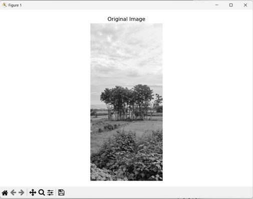
mahotas.pftas() 函式

mahotas.pftas() 函式接收影像和閾值作為輸入。它返回包含閾值鄰域統計資訊的列表。

語法

以下是 mahotas 中 pftas() 函式的基本語法：

mahotas.features.pftas(img, T={mahotas.threshold.otsu(img)})

其中：

• img - 輸入影像。

• T (可選) - 它定義了 TAS 中使用的閾值演算法（預設情況下它使用 Otsu 方法）。

示例

在下面的示例中，我們使用 mh.pftas() 函式計算影像的 TAS。

import mahotas as mh
import numpy as np
import matplotlib.pyplot as mtplt
# Loading the images
image = mh.imread('nature.jpeg')
# Converting it to grayscale
image = mh.colors.rgb2gray(image).astype(np.uint8)
# Computing parameter free TAS
pftas = mh.features.pftas(image)
# Printing the parameter free TAS value
print(pftas)
# Creating a figure and axes for subplots
fig, axes = mtplt.subplots(1, 1)
# Displaying the original image
axes.imshow(image, cmap='gray')
axes.set_title('Original Image')
axes.set_axis_off()
# Adjusting spacing between subplots
mtplt.tight_layout()
# Showing the figures
mtplt.show()

輸出

以下是上述程式碼的輸出：

[9.57767091e-01 1.48210628e-02  8.58153775e-03  1.18217967e-02
3.89970314e-03  1.86659948e-03  7.82131473e-04  3.19863291e-04
1.40214046e-04  9.73817262e-01  1.23385295e-02  5.89271152e-03
4.39412383e-03  1.90987201e-03  8.34387151e-04  4.60922081e-04
2.31642892e-04  1.20548852e-04  9.77691695e-01  8.29460231e-03
3.91949031e-03  7.21369229e-03  1.68522833e-03  7.53014919e-04
3.10737802e-04  1.12475646e-04  1.90636688e-05  9.47186804e-01
1.14563743e-02  9.65510102e-03  1.76918166e-02  5.35205921e-03
3.38515157e-03  2.13944340e-03  1.88754119e-03  1.24570817e-03
9.80623501e-01  3.72244140e-03  2.75392589e-03  4.22681210e-03
2.28359248e-03  1.92155953e-03  1.72971300e-03  1.63378974e-03
1.10466466e-03  9.59139669e-01  7.94832237e-03  7.15439233e-03
1.68349257e-02  3.75312384e-03  1.74123294e-03  9.83390623e-04
1.06007705e-03  1.38486661e-03]

獲得的影像是：

使用平均閾值

我們還可以使用平均閾值來計算影像的閾值鄰域統計。平均閾值是指透過取影像的平均畫素強度值來計算的閾值。

簡單來說，閾值是透過將影像中所有畫素的強度值相加，然後將該總和除以影像中畫素的總數來計算的。

在 mahotas 中，我們首先使用 mean() 函式計算平均閾值。然後，我們將此值設定為 pftas() 函式的 T 引數中，以使用平均閾值計算 TAS。

示例

在這裡，我們使用平均閾值獲取影像的 TAS。

import mahotas as mh
import numpy as np
import matplotlib.pyplot as mtplt
# Loading the images
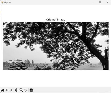
image = mh.imread('tree.tiff')
# Converting it to grayscale
image = mh.colors.rgb2gray(image).astype(np.uint8)
# Calculating threshold value
threshold = image > np.mean(image)
# Computing parameter free TAS using mean threshold
pftas = mh.features.pftas(image, threshold)
# Printing the parameter free TAS value
print(pftas)
# Creating a figure and axes for subplots
fig, axes = mtplt.subplots(1, 1)
# Displaying the original image
axes.imshow(image, cmap='gray')
axes.set_title('Original Image')
axes.set_axis_off()
# Adjusting spacing between subplots
mtplt.tight_layout()
# Showing the figures
mtplt.show()

輸出

執行上述程式碼後，我們得到以下輸出：

[0.63528106  0.07587514  0.06969174 0.07046435 0.05301355 0.0396411
 0.0278772   0.0187047   0.00945114 0.51355051 0.10530301 0.0960256
 0.08990634  0.06852526  0.05097649 0.03778379 0.02519265 0.01273634
 0.69524747  0.0985423   0.07691423 0.05862548 0.03432296 0.01936853
 0.01058033  0.00482901  0.00156968 0.46277808 0.17663377 0.13243407
 0.10085554  0.06345864  0.03523172 0.01735837 0.00835911 0.00289069
 0.78372479  0.0746143   0.04885744 0.03739208 0.02555628 0.01563048
 0.00822543  0.00436208  0.00163713 0.70661663 0.07079426 0.05897885
 0.06033083  0.04280415  0.02972053 0.01632203 0.01043743 0.00399529]

輸出影像是：