Mahotas - 計算線性二值模式

---

---

線性二值模式 (LBP) 用於分析影像中的模式。它將影像中中心畫素的強度值與其相鄰畫素進行比較，並將結果編碼成二進位制模式（0 或 1）。

想象一下，您有一幅灰度影像，其中每個畫素代表從黑色到白色的灰色陰影。LBP 將影像劃分為小區域。

對於每個區域，它都會檢視中心畫素並將其亮度與相鄰畫素進行比較。

如果相鄰畫素的亮度高於或等於中心畫素，則將其分配值為 1；否則，將其分配值為 0。此過程對所有相鄰畫素重複，從而建立二進位制模式。

在 Mahotas 中計算線性二值模式

在 Mahotas 中，我們可以使用 **features.lbp()** 函式計算影像中的線性二值模式。該函式將中心畫素的亮度與其鄰居進行比較，並根據比較結果分配二進位制值（0 或 1）。

然後將這些二進位制值組合起來，建立描述每個區域紋理的二進位制模式。透過對所有區域執行此操作，將建立一個直方圖以統計影像中每個模式的出現次數。

直方圖有助於我們瞭解影像中紋理的分佈。

mahotas.features.lbp() 函式

mahotas.features.lbp() 函式將灰度影像作為輸入，並返回每個畫素的二進位制值。然後使用二進位制值建立線性二值模式的直方圖。

直方圖的 x 軸表示計算出的 LBP 值，而 y 軸表示 LBP 值的頻率。

語法

以下是 mahotas 中 lbp() 函式的基本語法：

mahotas.features.lbp(image, radius, points, ignore_zeros=False)

其中，

• **image** - 輸入灰度影像。

• **radius** - 指定用於比較畫素強度的區域的大小。

• **points** - 確定計算每個畫素的 LBP 時應考慮的相鄰畫素數量。

• **ignore_zeros (可選)** - 一個標誌，指定是否忽略零值畫素（預設值為 false）。

示例

在以下示例中，我們使用 mh.features.lbp() 函式計算線性二值模式。

import mahotas as mh
import numpy as np
import matplotlib.pyplot as mtplt
# Loading the image
image = mh.imread('nature.jpeg')
# Converting it to grayscale
image = mh.colors.rgb2gray(image)
# Computing linear binary patterns
lbp = mh.features.lbp(image, 5, 5)
# Creating a figure and axes for subplots
fig, axes = mtplt.subplots(1, 2)
# Displaying the original image
axes[0].imshow(image, cmap='gray')
axes[0].set_title('Original Image')
axes[0].set_axis_off()
# Displaying the linear binary patterns
axes[1].hist(lbp)
axes[1].set_title('Linear Binary Patterns')
axes[1].set_xlabel('LBP Value')
axes[1].set_ylabel('Frequency')
# Adjusting spacing between subplots
mtplt.tight_layout()
# Showing the figures
mtplt.show()

輸出

以下是上述程式碼的輸出：

忽略零值畫素

在計算線性二值模式時，我們可以忽略零值畫素。零值畫素是指強度值為 0 的畫素。

它們通常表示影像的背景，但也可能表示噪聲。在灰度影像中，零值畫素由顏色“黑色”表示。

在 mahotas 中，我們可以將 **ignore_zeros** 引數設定為布林值“True”以在 mh.features.lbp() 函式中排除零值畫素。

示例

以下示例顯示了透過忽略零值畫素計算線性二值模式。

import mahotas as mh
import numpy as np
import matplotlib.pyplot as mtplt
# Loading the image
image = mh.imread('sea.bmp')
# Converting it to grayscale
image = mh.colors.rgb2gray(image)
# Computing linear binary patterns
lbp = mh.features.lbp(image, 20, 10, ignore_zeros=True)
# Creating a figure and axes for subplots
fig, axes = mtplt.subplots(1, 2)
# Displaying the original image
axes[0].imshow(image, cmap='gray')
axes[0].set_title('Original Image')
axes[0].set_axis_off()
# Displaying the linear binary patterns
axes[1].hist(lbp)
axes[1].set_title('Linear Binary Patterns')
axes[1].set_xlabel('LBP Value')
axes[1].set_ylabel('Frequency')
# Adjusting spacing between subplots
mtplt.tight_layout()
# Showing the figures
mtplt.show()

輸出

上述程式碼的輸出如下：

特定區域的 LBP

我們還可以計算影像中特定區域的線性二值模式。特定區域是指具有任何尺寸的影像的一部分。可以透過裁剪原始影像獲得。

在 mahotas 中，要計算特定區域的線性二值模式，我們首先需要從影像中找到感興趣的區域。為此，我們分別為 x 和 y 座標指定起始和結束畫素值。然後，我們可以使用 lbp() 函式計算該區域的 LBP。

例如，如果我們將值指定為 [300:800]，則該區域將從第 300 個畫素開始，並在垂直方向（y 軸）上一直延伸到第 800 個畫素。

示例

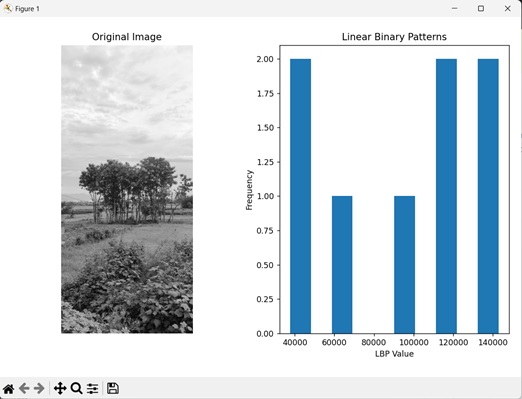
這裡，我們正在計算指定灰度影像的特定部分的 LBP。

import mahotas as mh
import numpy as np
import matplotlib.pyplot as mtplt
# Loading the image
image = mh.imread('tree.tiff')
# Converting it to grayscale
image = mh.colors.rgb2gray(image)
# Specifying a region of interest
image = image[300:800]
# Computing linear binary patterns
lbp = mh.features.lbp(image, 20, 10)
# Creating a figure and axes for subplots
fig, axes = mtplt.subplots(1, 2)
# Displaying the original image
axes[0].imshow(image, cmap='gray')
axes[0].set_title('Original Image')
axes[0].set_axis_off()
# Displaying the linear binary patterns
axes[1].hist(lbp)
axes[1].set_title('Linear Binary Patterns')
axes[1].set_xlabel('LBP Value')
axes[1].set_ylabel('Frequency')
# Adjusting spacing between subplots
mtplt.tight_layout()
# Showing the figures
mtplt.show()

輸出

執行上述程式碼後，我們將獲得以下輸出：