Mahotas - 裁剪影像

---

---

裁剪影像指的是從影像中選擇和提取特定的感興趣區域，並丟棄其餘部分。它允許我們專注於影像中特定區域或物件，同時移除不相關或不需要的部分。

一般來說，要裁剪影像，您需要定義要保留區域的座標或尺寸。

在 Mahotas 中裁剪影像

要使用 Mahotas 裁剪影像，我們可以使用 NumPy 陣列切片操作來選擇影像的所需區域。我們需要定義所需 ROI 的座標或尺寸。這可以透過指定要裁剪區域的起點、寬度和高度來完成。

透過提取和隔離 ROI，我們可以僅分析、操作或顯示影像的相關部分。

示例

在以下示例中，我們將影像裁剪到所需的大小 -

import mahotas as mh
import numpy as np
import matplotlib.pyplot as plt
image = mh.imread('sun.png')
cropping= image[50:1250,40:340]
# Create a figure with subplots
fig, axes = plt.subplots(1, 2, figsize=(10, 5))
# Display the original image
axes[0].imshow(image)
axes[0].set_title('Original Image')
axes[0].axis('off')
# Display the cropped image
axes[1].imshow(cropping, cmap='gray')
axes[1].set_title('Cropped Image')
axes[1].axis('off')
# Adjust the layout and display the plot
plt.tight_layout()
plt.show()

輸出

以下是上述程式碼的輸出 -

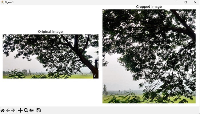
裁剪正方形區域

要在 mahotas 中裁剪正方形區域，我們需要確定起始和結束行以及列。以下是如何計算這些值的方法 -

步驟 1 - 找到影像的最小尺寸。

步驟 2 - 透過從總行數中減去最小尺寸並將結果除以 2 來計算起始行。

步驟 3 - 透過將起始行新增到最小尺寸來計算結束行。

步驟 4 - 使用類似的方法計算起始列。

步驟 5 - 透過將起始列新增到最小尺寸來計算結束列。

使用計算出的起始和結束行以及列，我們可以從影像中裁剪正方形區域。我們透過使用適當的行和列範圍對影像陣列進行索引來實現這一點。

示例

在這裡，我們嘗試在正方形區域中裁剪影像 -

import mahotas as mh
import numpy as np
import matplotlib.pyplot as plt
image = mh.imread('tree.tiff')
# Get the minimum dimension
size = min(image.shape[:2])
# Calculating the center of the image
center = tuple(map(lambda x: x // 2, image.shape[:2]))
# Cropping a square region around the center
crop = image[center[0] - size // 2:center[0] + size // 2, center[1] - size //
2:center[1] + size // 2]
# Create a figure with subplots
fig, axes = plt.subplots(1, 2, figsize=(10, 5))
# Display the original image
axes[0].imshow(image)
axes[0].set_title('Original Image')
axes[0].axis('off')
# Display the cropped image
axes[1].imshow(crop, cmap='gray')
axes[1].set_title('Cropped Image')
axes[1].axis('off')
# Adjust the layout and display the plot
plt.tight_layout()
plt.show()

輸出

執行上述程式碼後，我們將獲得以下輸出 -

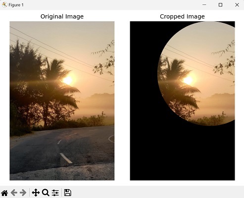
裁剪圓形區域

要在 mahotas 中將影像裁剪為圓形區域，我們需要確定圓心的座標和半徑。

我們可以透過將中心計算為影像尺寸的中點並將半徑設定為最小尺寸的一半來實現。

接下來，我們建立一個與影像尺寸相同的布林掩碼，其中 True 值表示圓形區域內的畫素。

我們透過計算每個畫素到中心的距離並在指定半徑內設定 True 來實現。

現在我們有了圓形掩碼，我們可以透過將圓形區域外的值設定為零將其應用於影像。最後，我們得到裁剪後的影像。

示例

現在，我們嘗試在圓形區域中裁剪影像 -

import mahotas as mh
import numpy as np
import matplotlib.pyplot as plt
image = mh.imread('sun.png')
# Calculating the center of the image
center = tuple(map(lambda x: x // 2, image.shape[:2]))
# Calculating the radius as half the minimum dimension
radius = min(image.shape[:2]) // 2
# Creating a boolean mask of zeros
mask = np.zeros(image.shape[:2], dtype=bool)
# Creating meshgrid indices
y, x = np.ogrid[:image.shape[0], :image.shape[1]]
# Setting mask values within the circular region to True
mask[(x - center[0])**2 + (y - center[1])**2 <= radius**2] = True
crop = image.copy()
# Setting values outside the circular region to zero
crop[~mask] = 0
# Create a figure with subplots
fig, axes = plt.subplots(1, 2, figsize=(7, 5))
# Display the original image
axes[0].imshow(image)
axes[0].set_title('Original Image')
axes[0].axis('off')
# Display the cropped image
axes[1].imshow(crop, cmap='gray')
axes[1].set_title('Cropped Image')
axes[1].axis('off')
# Adjust the layout and display the plot
plt.tight_layout()
plt.show()

輸出

獲得的輸出如下所示 -