- Matlab 教程
- MATLAB - 首頁
- MATLAB - 概述
- MATLAB - 特性
- MATLAB - 環境設定
- MATLAB - 編輯器
- MATLAB - 線上版
- MATLAB - 工作區
- MATLAB - 語法
- MATLAB - 變數
- MATLAB - 命令
- MATLAB - 資料型別
- MATLAB - 運算子
- MATLAB - 日期和時間
- MATLAB - 數字
- MATLAB - 隨機數
- MATLAB - 字串和字元
- MATLAB - 文字格式化
- MATLAB - 時間表
- MATLAB - M 檔案
- MATLAB - 冒號表示法
- MATLAB - 資料匯入
- MATLAB - 資料匯出
- MATLAB - 資料歸一化
- MATLAB - 預定義變數
- MATLAB - 決策
- MATLAB - 決策語句
- MATLAB - if 語句
- MATLAB - if-else 語句
- MATLAB - if-elseif-else 語句
- MATLAB - 巢狀 if 語句
- MATLAB - switch 語句
- MATLAB - 巢狀 switch
- MATLAB - 迴圈
- MATLAB - 迴圈
- MATLAB - for 迴圈
- MATLAB - while 迴圈
- MATLAB - 巢狀迴圈
- MATLAB - break 語句
- MATLAB - continue 語句
- MATLAB - end 語句
- MATLAB - 陣列
- MATLAB - 陣列
- MATLAB - 向量
- MATLAB - 轉置運算子
- MATLAB - 陣列索引
- MATLAB - 多維陣列
- MATLAB - 相容陣列
- MATLAB - 分類陣列
- MATLAB - 元胞陣列
- MATLAB - 矩陣
- MATLAB - 稀疏矩陣
- MATLAB - 表格
- MATLAB - 結構體
- MATLAB - 陣列乘法
- MATLAB - 陣列除法
- MATLAB - 陣列函式
- MATLAB - 函式
- MATLAB - 函式
- MATLAB - 函式引數
- MATLAB - 匿名函式
- MATLAB - 巢狀函式
- MATLAB - return 語句
- MATLAB - 無返回值函式
- MATLAB - 區域性函式
- MATLAB - 全域性變數
- MATLAB - 函式控制代碼
- MATLAB - 濾波器函式
- MATLAB - 階乘
- MATLAB - 私有函式
- MATLAB - 子函式
- MATLAB - 遞迴函式
- MATLAB - 函式優先順序順序
- MATLAB - map 函式
- MATLAB - mean 函式
- MATLAB - end 函式
- MATLAB - 錯誤處理
- MATLAB - 錯誤處理
- MATLAB - try...catch 語句
- MATLAB - 除錯
- MATLAB - 繪圖
- MATLAB - 繪圖
- MATLAB - 繪製陣列
- MATLAB - 繪製向量
- MATLAB - 條形圖
- MATLAB - 直方圖
- MATLAB - 圖形
- MATLAB - 二維線圖
- MATLAB - 三維圖
- MATLAB - 格式化繪圖
- MATLAB - 對數座標軸繪圖
- MATLAB - 繪製誤差條
- MATLAB - 繪製三維等高線圖
- MATLAB - 極座標圖
- MATLAB - 散點圖
- MATLAB - 繪製表示式或函式
- MATLAB - 繪製矩形
- MATLAB - 繪製頻譜圖
- MATLAB - 繪製網格曲面
- MATLAB - 繪製正弦波
- MATLAB - 插值
- MATLAB - 插值
- MATLAB - 線性插值
- MATLAB - 二維陣列插值
- MATLAB - 三維陣列插值
- MATLAB - 多項式
- MATLAB - 多項式
- MATLAB - 多項式加法
- MATLAB - 多項式乘法
- MATLAB - 多項式除法
- MATLAB - 多項式的導數
- MATLAB - 變換
- MATLAB - 變換函式
- MATLAB - 拉普拉斯變換
- MATLAB - 拉普拉斯濾波器
- MATLAB - 高斯-拉普拉斯濾波器
- MATLAB - 逆傅立葉變換
- MATLAB - 傅立葉變換
- MATLAB - 快速傅立葉變換
- MATLAB - 二維逆餘弦變換
- MATLAB - 向座標軸新增圖例
- MATLAB - 面向物件
- MATLAB - 面向物件程式設計
- MATLAB - 類和物件
- MATLAB - 函式過載
- MATLAB - 運算子過載
- MATLAB - 使用者自定義類
- MATLAB - 複製物件
- MATLAB - 代數
- MATLAB - 線性代數
- MATLAB - 高斯消去法
- MATLAB - 高斯-約旦消去法
- MATLAB - 簡化行階梯形
- MATLAB - 特徵值和特徵向量
- MATLAB - 積分
- MATLAB - 積分
- MATLAB - 二重積分
- MATLAB - 梯形法則
- MATLAB - 辛普森法則
- MATLAB - 其他
- MATLAB - 微積分
- MATLAB - 微分
- MATLAB - 矩陣的逆
- MATLAB - GNU Octave
- MATLAB - Simulink
- MATLAB - 有用資源
- MATLAB - 快速指南
- MATLAB - 有用資源
- MATLAB - 討論
MATLAB - 線性插值
線性插值是一種用於估計兩個已知資料點之間值的方法。在這種方法中,在兩點之間畫一條直線,然後根據端點的已知值計算沿線任何中間點的值。線性插值常用於各種應用,例如訊號處理、計算機圖形學和資料分析,以根據一組已知資料點估計未知值。
語法
vq = interp1(x,v,xq)
vq = interp1(x,v,xq,method)
vq = interp1(x,v,xq,method,extrapolation)
vq = interp1(v,xq)
以下是語法的解釋:
vq = interp1(x,v,xq) - 透過估計 v 中現有資料點之間的點來計算新的值 vq。已知點由 x 和 v 指定,其中 x 是取樣點,v 是相應的值。該函式計算由 xq 指定的位置的值。如果 v 包含在相同點取樣的多組資料,則 v 的每一列都代表一組不同的樣本值。
vq = interp1(x,v,xq,method) - 允許您為插值選擇特定方法。method 引數指定函式應如何估計已知點之間的值。可用方法包括 'linear'、'nearest'、'next'、'previous'、'pchip'、'cubic'、'v5cubic'、'makima' 或 'spline'。預設方法是 'linear',它在點之間建立一條直線。
vq = interp1(x,v,xq,method,extrapolation) - 允許您指定如何處理位於已知資料點 x 範圍之外的點。如果將 extrapolation 設定為 'extrap',則該函式將使用指定的插值方法來估計範圍之外的點的值。或者,您可以指定單個值,interp1() 將為 x 範圍之外的所有點返回該值。
vq = interp1(v,xq) - 假設一組預設的取樣點座標來計算插值值。預設座標是從 1 到 n 的數字序列,其中 n 取決於 v 的形狀:
- 如果 v 是向量,則預設座標是從 1 到 v 的長度。
- 如果 v 是陣列,則預設座標是從 1 到 v 的行數。
MATLAB 中線性插值的示例
以下是一些 MATLAB 中線性插值的常見示例:
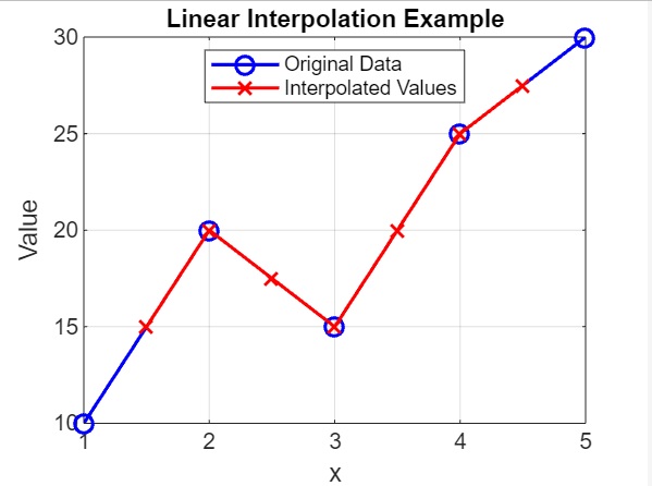
示例 1:使用 vq = interp1(x,v,xq)
我們的程式碼如下:
x = [1, 2, 3, 4, 5];
v = [10, 20, 15, 25, 30];
xq = 1.5:0.5:4.5;

% Perform linear interpolation
vq = interp1(x, v, xq);

% Plot the original data points
figure;
plot(x, v, 'bo-', 'LineWidth', 1.5, 'MarkerSize', 8);
hold on;

% Plot the interpolated values
plot(xq, vq, 'rx-', 'LineWidth', 1.5, 'MarkerSize', 8);

% Add labels and legend
xlabel('x');
ylabel('Value');
title('Linear Interpolation Example');
legend('Original Data', 'Interpolated Values', 'Location', 'best');
grid on;
hold off;
在這個例子中:
- 我們將 x 定義為取樣點 [1, 2, 3, 4, 5],並將 v 定義為相應的值 [10, 20, 15, 25, 30]。
- xq 定義為插值的查詢點,範圍從 1.5 到 4.5,步長為 0.5。
- interp1() 函式用於根據已知點 (x, v) 插值 xq 查詢點的值。
- 計算並顯示插值值 vq。vq 的每個元素都對應於 xq 中相應查詢點的插值值。
- 該程式碼將原始資料點繪製為由線連線的藍色圓圈 ('bo-'),並將插值值繪製為由線連線的紅色十字 ('rx-')。
程式碼執行後,輸出如下:
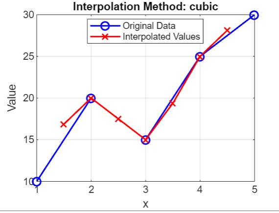
示例 2:使用 vq = interp1(x,v,xq,method),其中 method 為 cubic
我們的程式碼是:
x = [1, 2, 3, 4, 5];
v = [10, 20, 15, 25, 30];

xq = 1.5:0.5:4.5;

% Perform interpolation with different methods

method = 'cubic';
vq = interp1(x, v, xq, method);

% Plot the interpolated values

plot(x, v, 'bo-', 'LineWidth', 1.5, 'MarkerSize', 8);
hold on;
plot(xq, vq, 'rx-', 'LineWidth', 1.5, 'MarkerSize', 8);
xlabel('x');
ylabel('Value');
title(['Interpolation Method: ', method]);
legend('Original Data', 'Interpolated Values', 'Location', 'best');
grid on;
hold off;
在上面的示例中,我們有:
- 我們將 x 定義為取樣點 [1, 2, 3, 4, 5],並將 v 定義為相應的值 [10, 20, 15, 25, 30]。
- 我們定義了用於插值的查詢點 xq,範圍從 1.5 到 4.5,步長為 0.5。
- 我們使用了 cubic 方法,可用的方法選項包括 'nearest'、'next'、'previous'、'linear'、'pchip'、'cubic'、'spline'。
- 我們使用 interp1() 計算插值值 vq,最後繪製 cubic 方法的原始資料點和插值值。原始資料點為藍色圓圈,插值值為紅色十字,標題指示所使用的插值方法。
執行後,我們得到的輸出是:
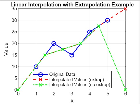
示例 3:使用 vq = interp1(x,v,xq,method,extrapolation) 進行外推
我們的程式碼如下:
x = [1, 2, 3, 4, 5];
v = [10, 20, 15, 25, 30];

xq = [0, 1.5, 2.5, 3.5, 4.5, 6];

% Perform linear interpolation with 'extrap' extrapolation
vq_extrap = interp1(x, v, xq, 'linear', 'extrap');

% Perform linear interpolation without extrapolation
vq_no_extrap = interp1(x, v, xq, 'linear', 0);

figure;
plot(x, v, 'bo-', 'LineWidth', 1.5, 'MarkerSize', 8);
hold on;

plot(xq, vq_extrap, 'rx--', 'LineWidth', 1.5, 'MarkerSize', 8);
plot(xq, vq_no_extrap, 'gx:', 'LineWidth', 1.5, 'MarkerSize', 8);

xlabel('x');
ylabel('Value');
title('Linear Interpolation with Extrapolation Example');
legend('Original Data', 'Interpolated Values (extrap)', 'Interpolated Values (no extrap)', 'Location', 'best');
grid on;
hold off;
在上面的示例中,我們有:
- 我們將 x 定義為取樣點 [1, 2, 3, 4, 5],並將 v 定義為相應的值 [10, 20, 15, 25, 30]。
- 我們定義了用於插值的查詢點 xq,包括一些超出 x 範圍的點(例如,0 和 6)。
- 我們使用 interp1() 計算具有 'extrap' 外推法的插值值 vq_extrap 和沒有外推法的 vq_no_extrap。
- 我們繪製原始資料點為藍色圓圈,vq_extrap 為具有虛線的紅色十字,vq_no_extrap 為具有點線的綠色十字。
程式碼執行後,我們得到的輸出如下:
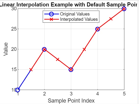
示例 4:使用 vq = interp1(v,xq) 的預設取樣點
我們的程式碼如下:
v = [10, 20, 15, 25, 30];

xq = 1.5:0.5:5.5;

% Perform linear interpolation assuming default sample point coordinates
vq = interp1(v, xq);

% Plot the original values and the interpolated values
figure;
plot(1:length(v), v, 'bo-', 'LineWidth', 1.5, 'MarkerSize', 8);
hold on;
plot(xq, vq, 'rx-', 'LineWidth', 1.5, 'MarkerSize', 8);
xlabel('Sample Point Index');
ylabel('Value');
title('Linear Interpolation Example with Default Sample Points');
legend('Original Values', 'Interpolated Values', 'Location', 'best');
grid on;
hold off;
在上面的例子中:
- 我們將 v 定義為用於插值的值 [10, 20, 15, 25, 30]。
- 我們定義了用於插值的查詢點 xq,範圍從 1.5 到 5.5,步長為 0.5。
- 我們使用 interp1() 計算假設預設取樣點座標的插值值 vq。
- 我們繪製原始值為由線連線的藍色圓圈,插值值為由線連線的紅色十字。x 軸表示取樣點的索引。
執行後,輸出為:
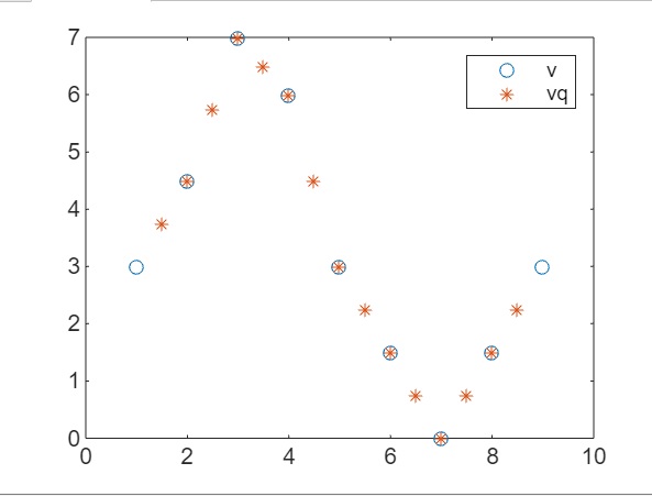
示例 5:無點的線性插值
我們的程式碼如下:
v = [3, 4.5, 7, 6, 3, 1.5, 0, 1.5, 3];
xq = 1.5:0.5:8.5;
vq = interp1(1:numel(v), v, xq);
figure
plot((1:9),v,'o',xq,vq,'*');
legend('v','vq');
在上面的程式碼中,我們有:
- v = [3, 4.5, 7, 6, 3, 1.5, 0, 1.5, 3]; - 定義一個向量 v,其中包含用於插值的原始值。
- xq = 1.5:0.5:8.5; - 定義用於插值的查詢點 xq。這些點的範圍是從 1.5 到 8.5,步長為 0.5。
- vq = interp1(1:numel(v), v, xq); - 使用 interp1 函式執行線性插值。該函式在 xq 中指定的查詢點處對 v 中的值進行插值。由於沒有明確指定取樣點,因此該函式使用從 1 到 v 中元素數量的預設取樣點座標。
- plot((1:9),v,'o',xq,vq,'*'); - 繪製原始值 v 為藍色圓圈,插值值 vq 為紅色星號。x 軸表示取樣點的索引。
執行後,我們得到的輸出如下:
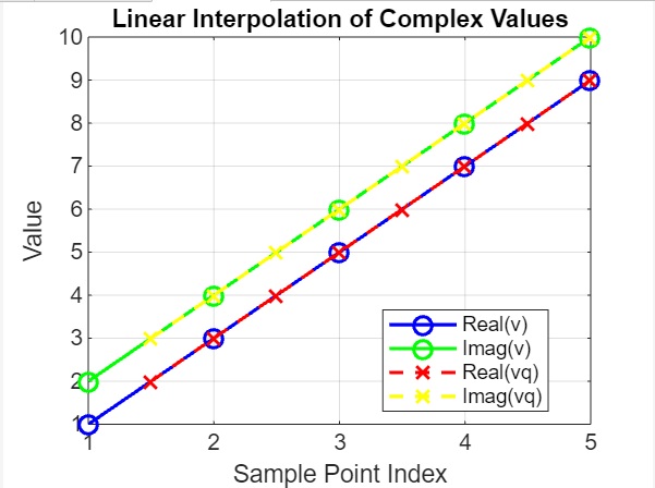
示例 6:使用複數
我們的程式碼如下:
v = [1+2i, 3+4i, 5+6i, 7+8i, 9+10i];

xq = 1.5:0.5:5.5;

% Perform linear interpolation
vq = interp1(1:numel(v), v, xq, 'linear');

% Plot the original and interpolated complex values
figure;
plot(1:numel(v), real(v), 'bo-', 1:numel(v), imag(v), 'go-', ...
   xq, real(vq), 'rx--', xq, imag(vq), 'yx--', 'LineWidth', 1.5, 'MarkerSize', 8);
xlabel('Sample Point Index');
ylabel('Value');
title('Linear Interpolation of Complex Values');
legend('Real(v)', 'Imag(v)', 'Real(vq)', 'Imag(vq)', 'Location', 'best');
grid on;
在上面的例子中:
- 我們定義一個包含複數值的向量 v。
- 我們定義用於插值的查詢點 xq。
- 我們使用 interp1 對查詢點 xq 處的複數值 v 執行線性插值。
- 我們繪製原始 (v) 和插值 (vq) 複數值的實部和虛部。x 軸表示取樣點的索引。
執行後,我們得到的輸出如下:
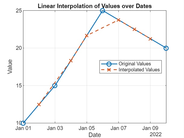
示例 7:使用日期和時間
我們的程式碼如下:
dates = datetime({'2022-01-01', '2022-01-03', '2022-01-06', '2022-01-10'}, 'InputFormat', 'yyyy-MM-dd');
values = [10, 15, 25, 20];

query_dates = datetime({'2022-01-02', '2022-01-04', '2022-01-05', '2022-01-07', '2022-01-08', '2022-01-09'}, 'InputFormat', 'yyyy-MM-dd');

% Perform linear interpolation
interp_values = interp1(dates, values, query_dates, 'linear');

% Plot the original and interpolated values
figure;
plot(dates, values, 'o-', query_dates, interp_values, 'x--', 'LineWidth', 1.5, 'MarkerSize', 8);
xlabel('Date');
ylabel('Value');
title('Linear Interpolation of Values over Dates');
legend('Original Values', 'Interpolated Values', 'Location', 'best');
grid on;
在上面的示例中:
- 我們定義一個向量 dates,其中包含表示日期的 datetime 值,以及一個包含數值的相應向量 values。
- 我們定義一個向量 query_dates,其中包含我們想要插值值的 datetime 值。
- 我們使用 interp1 對原始值在日期上進行線性插值,以估計 query_dates 的值。
- 我們繪製原始值和日期上的插值值。x 軸表示日期,y 軸表示值。
執行後,我們得到的輸出如下:
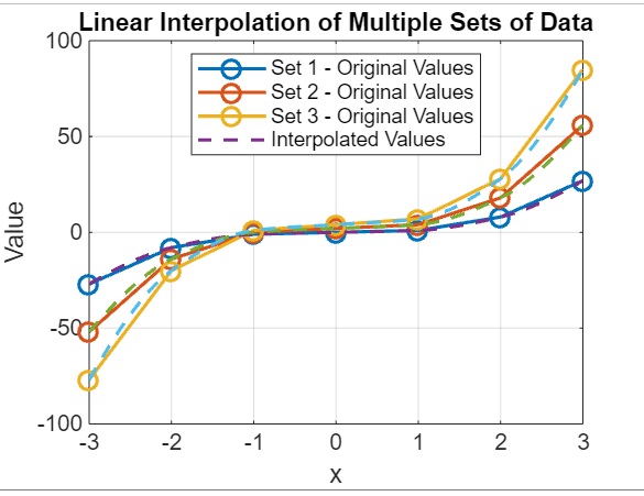
示例 8:多組資料
我們的程式碼如下:
x = (-3:3)';
v1 = x.^3;
v2 = 2*x.^3 + 2;
v3 = 3*x.^3 + 4;

v = [v1 v2 v3];

xq = -3:0.1:3;

vq = interp1(x, v, xq, 'pchip');

% Plot the original and interpolated values for all three sets of data
figure;
plot(x, v, 'o-', xq, vq, '--', 'LineWidth', 1.5, 'MarkerSize', 8);
xlabel('x');
ylabel('Value');
title('Linear Interpolation of Multiple Sets of Data');
legend('Set 1 - Original Values', 'Set 2 - Original Values', 'Set 3 - Original Values', 'Interpolated Values', 'Location', 'best');
grid on;
在上面的示例中:
- 我們定義一個向量 x,表示原始取樣點。
- 我們使用 x 的不同函式計算三組原始值 (v1、v2、v3)。
- 我們將原始值組合到一個矩陣 v 中。
- 我們定義一個向量 xq,其中包含用於插值的查詢點。
- 我們使用 interp1 函式和 'pchip' 方法對樣本點的原始值進行插值,以估算查詢點的值。
- 我們繪製了所有三組資料的原始值和插值值。x 軸表示 x,y 軸表示值。
執行後,我們得到的輸出如下: