機器學習 - 均值漂移聚類

---

---

均值漂移聚類演算法是一種非引數聚類演算法，它透過迭代地將資料點的均值移動到資料最密集的區域來工作。資料的最密集區域由核函式確定，核函式是根據資料點到均值的距離為資料點分配權重的函式。均值漂移聚類中使用的核函式通常是高斯函式。

均值漂移聚類演算法涉及的步驟如下：

• 將每個資料點的均值初始化為其自身的值。

• 對於每個資料點，計算均值漂移向量，該向量指向資料最密集的區域。

• 透過將每個資料點的均值移動到資料最密集的區域來更新每個資料點的均值。

• 重複步驟2和3，直到達到收斂。

均值漂移聚類演算法是一種基於密度的聚類演算法，這意味著它根據資料點的密度而不是它們之間的距離來識別聚類。換句話說，該演算法根據資料點密度最高的區域來識別聚類。

在Python中實現均值漂移聚類

可以使用scikit-learn庫在Python程式語言中實現均值漂移聚類演算法。scikit-learn庫是Python中一個流行的機器學習庫，它提供了各種用於資料分析和機器學習的工具。以下步驟涉及在Python中使用scikit-learn庫實現均值漂移聚類演算法：

步驟1 - 匯入必要的庫

numpy庫用於Python中的科學計算，而matplotlib庫用於資料視覺化。sklearn.cluster庫包含MeanShift類，該類用於在Python中實現均值漂移聚類演算法。

estimate_bandwidth函式用於估計核函式的頻寬，這是均值漂移聚類演算法中的一個重要引數。

import numpy as np
import matplotlib.pyplot as plt
from sklearn.cluster import MeanShift, estimate_bandwidth

步驟2 - 生成資料

在此步驟中，我們生成一個包含500個數據點和2個特徵的隨機資料集。我們使用numpy.random.randn函式生成資料。

# Generate the data
X = np.random.randn(500,2)

步驟3 - 估計核函式的頻寬

在此步驟中，我們使用estimate_bandwidth函式估計核函式的頻寬。頻寬是均值漂移聚類演算法中的一個重要引數，它確定了核函式的寬度。

# Estimate the bandwidth
bandwidth = estimate_bandwidth(X, quantile=0.1, n_samples=100)

步驟4 - 初始化均值漂移聚類演算法

在此步驟中，我們使用MeanShift類初始化均值漂移聚類演算法。我們將頻寬引數傳遞給該類以設定核函式的寬度。

# Initialize the Mean-Shift algorithm
ms = MeanShift(bandwidth=bandwidth, bin_seeding=True)

步驟5 - 訓練模型

在此步驟中，我們使用MeanShift類的fit方法在資料集上訓練均值漂移聚類演算法。

# Train the model
ms.fit(X)

步驟6 - 視覺化結果

# Visualize the results
labels = ms.labels_
cluster_centers = ms.cluster_centers_
n_clusters_ = len(np.unique(labels))
print("Number of estimated clusters:", n_clusters_)

# Plot the data points and the centroids
plt.figure(figsize=(7.5, 3.5))
plt.scatter(X[:,0], X[:,1], c=labels, cmap='viridis')
plt.scatter(cluster_centers[:,0], cluster_centers[:,1], marker='*', s=300, c='r')
plt.show()

在此步驟中，我們視覺化均值漂移聚類演算法的結果。我們從訓練好的模型中提取聚類標籤和聚類中心。然後，我們列印估計的聚類數量。最後，我們使用matplotlib庫繪製資料點和質心。

示例

以下是Python中均值漂移聚類演算法的完整實現示例：

import numpy as np
import matplotlib.pyplot as plt
from sklearn.cluster import MeanShift, estimate_bandwidth

# Generate the data
X = np.random.randn(500,2)

# Estimate the bandwidth
bandwidth = estimate_bandwidth(X, quantile=0.1, n_samples=100)

# Initialize the Mean-Shift algorithm
ms = MeanShift(bandwidth=bandwidth, bin_seeding=True)

# Train the model
ms.fit(X)

# Visualize the results
labels = ms.labels_
cluster_centers = ms.cluster_centers_
n_clusters_ = len(np.unique(labels))
print("Number of estimated clusters:", n_clusters_)

# Plot the data points and the centroids
plt.figure(figsize=(7.5, 3.5))
plt.scatter(X[:,0], X[:,1], c=labels, cmap='summer')
plt.scatter(cluster_centers[:,0], cluster_centers[:,1], marker='*',
s=200, c='r')
plt.show()

輸出

執行程式時，它將生成以下繪圖作為輸出：

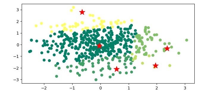
均值漂移聚類的應用

均值漂移聚類演算法在各個領域都有多種應用。均值漂移聚類的一些應用如下：

• 計算機視覺 - 均值漂移聚類廣泛用於計算機視覺中的物體跟蹤、影像分割和特徵提取。

• 影像處理 - 均值漂移聚類用於影像分割，即根據畫素的相似性將影像劃分為多個片段的過程。

• 異常檢測 - 均值漂移聚類可用於透過識別低密度區域來檢測資料中的異常。

• 客戶細分 - 均值漂移聚類可用於透過識別具有相似行為和偏好的客戶群體來進行營銷中的客戶細分。

• 社交網路分析 - 均值漂移聚類可用於根據使用者的興趣和互動對社交網路中的使用者進行聚類。