機器學習 - 資料分佈

在機器學習中，資料分佈指的是資料點在一個數據集中分佈或分散的方式。瞭解資料集中資料的分佈非常重要，因為它會對機器學習演算法的效能產生重大影響。

資料分佈可以通過幾個統計量來描述，包括均值、中位數、眾數、標準差和方差。這些度量有助於描述資料的集中趨勢、離散程度和形狀。

下面列出了一些機器學習中常見的資料分佈型別：

正態分佈

正態分佈，也稱為高斯分佈，是一種在機器學習和統計學中廣泛使用的連續機率分佈。它是一個鐘形曲線，描述了一個隨機變數的機率分佈，該變數圍繞均值對稱。正態分佈有兩個引數，均值 (μ) 和標準差 (σ)。

在機器學習中，正態分佈通常用於模擬線性迴歸和其他統計模型中誤差項的分佈。它也用作各種假設檢驗和置信區間的基礎。

正態分佈的一個重要特性是經驗法則，也稱為 68-95-99.7 法則。該法則指出，大約 68% 的觀測值落在均值的一個標準差內，95% 的觀測值落在均值的兩個標準差內，99.7% 的觀測值落在均值的三個標準差內。

Python 提供了各種庫，可用於處理正態分佈。其中一個庫是 **scipy.stats**，它提供了用於計算正態分佈的機率密度函式 (PDF)、累積分佈函式 (CDF)、百分位函式 (PPF) 和隨機變數的函式。

示例

以下是如何使用 **scipy.stats** 生成和視覺化正態分佈的示例：

import numpy as np
from scipy.stats import norm
import matplotlib.pyplot as plt

# Generate a random sample of 1000 values from a normal distribution
mu = 0 # Mean
sigma = 1 # Standard deviation
sample = np.random.normal(mu, sigma, 1000)

# Calculate the PDF for the normal distribution
x = np.linspace(mu - 3*sigma, mu + 3*sigma, 100)
pdf = norm.pdf(x, mu, sigma)
# Plot the histogram of the random sample and the PDF of the normal
distribution
plt.figure(figsize=(7.5, 3.5))
plt.hist(sample, bins=30, density=True, alpha=0.5)
plt.plot(x, pdf)
plt.show()

在這個例子中，我們首先使用 **np.random.normal** 從均值為 0、標準差為 1 的正態分佈中生成 1000 個隨機值的樣本。然後，我們使用 norm.pdf 計算正態分佈的 PDF，並使用 **np.linspace** 生成一個包含 100 個從 μ -3σ 到 μ +3σ 的均勻間隔值的陣列。

最後，我們使用 **plt.hist** 繪製隨機樣本的直方圖，並使用 **plt.plot** 在上面疊加正態分佈的 PDF。

輸出

生成的圖表顯示了正態分佈的鐘形曲線以及近似於正態分佈的隨機樣本的直方圖。

偏態分佈

在機器學習中，偏態分佈指的是資料集在其均值或平均值周圍分佈不均勻。在偏態分佈中，大多數資料點傾向於聚集在分佈的一端，而另一端的資料點較少。

偏態分佈有兩種型別：左偏和右偏。左偏分佈，也稱為負偏分佈，在分佈的左側有一個長尾，大多數資料點在右側。相反，右偏分佈，也稱為正偏分佈，在分佈的右側有一個長尾，大多數資料點在左側。

偏態分佈可能出現在許多不同型別的資料集中，例如財務資料、社交媒體指標或醫療記錄。在機器學習中，識別並正確處理偏態分佈非常重要，因為它們會影響某些演算法和模型的效能。例如，在某些情況下，偏態資料會導致預測偏差和結果不準確，可能需要進行歸一化或資料轉換等預處理技術來提高模型的效能。

示例

以下是如何使用 Python 的 NumPy 和 Matplotlib 庫生成和繪製偏態分佈的示例：

import numpy as np
import matplotlib.pyplot as plt

# Generate a skewed distribution using NumPy's random function
data = np.random.gamma(2, 1, 1000)

# Plot a histogram of the data to visualize the distribution
plt.figure(figsize=(7.5, 3.5))
plt.hist(data, bins=30)

# Add labels and title to the plot
plt.xlabel('Value')
plt.ylabel('Frequency')
plt.title('Skewed Distribution')

# Show the plot
plt.show()

輸出

執行此程式碼後，您將獲得以下圖表作為輸出：

均勻分佈

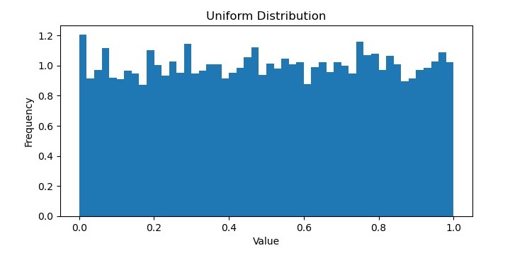
在機器學習中，均勻分佈指的是所有可能的結果都等可能發生的機率分佈。換句話說，資料集中每個值都有相同的被觀察到的機率，並且資料點沒有圍繞特定值聚集。

均勻分佈通常用作與其他分佈進行比較的基線，因為它表示資料的隨機和無偏取樣。它在某些型別的應用中也很有用，例如生成隨機數或從集合中無偏地選擇專案。

在機率論中，連續均勻分佈的機率密度函式定義為：

$$f\left ( x \right )=\left\{\begin{matrix} 1 & for\: a\leq x\leq b \\ 0 & otherwise \\ \end{matrix}\right.$$

其中 a 和 b 分別是分佈的最小值和最大值。均勻分佈的均值為 $\frac{a+b}{2} $，方差為 $\frac{\left ( b-a \right )^{2}}{12}$

示例

在 Python 中，NumPy 庫提供了用於從均勻分佈生成隨機數的函式，例如 **numpy.random.uniform()**。這些函式將分佈的最小值和最大值作為引數，可用於生成具有均勻分佈的資料集。

以下是如何使用 Python 的 NumPy 庫生成均勻分佈的示例：

import numpy as np
import matplotlib.pyplot as plt

# Generate 10,000 random numbers from a uniform distribution between 0 and 1
uniform_data = np.random.uniform(low=0, high=1, size=10000)

# Plot the histogram of the uniform data
plt.figure(figsize=(7.5, 3.5))
plt.hist(uniform_data, bins=50, density=True)

# Add labels and title to the plot
plt.xlabel('Value')
plt.ylabel('Frequency')
plt.title('Uniform Distribution')

# Show the plot
plt.show()

輸出

它將生成以下圖表作為輸出：

雙峰分佈

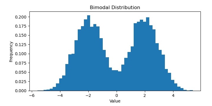
在機器學習中，雙峰分佈是一種具有兩個不同眾數或峰值的機率分佈。換句話說，分佈有兩個資料值最有可能出現的位置，它們之間存在一個數據不太可能出現的谷或槽。

雙峰分佈可能出現在各種型別的資料中，例如生物識別測量、經濟指標或社交媒體指標。它們可以表示資料集中不同的子群體，或隨時間推移的不同行為模式或趨勢。

可以使用各種統計方法識別和分析雙峰分佈，例如直方圖、核密度估計或假設檢驗。在某些情況下，雙峰分佈可以擬合到特定的機率分佈，例如高斯混合模型，該模型允許分別對底層子群體進行建模。

示例

在 Python 中，NumPy、SciPy 和 Matplotlib 等庫提供了用於生成和視覺化雙峰分佈的函式。

例如，以下程式碼生成並繪製了一個雙峰分佈：

import numpy as np
import matplotlib.pyplot as plt

# Generate 10,000 random numbers from a bimodal distribution
bimodal_data = np.concatenate((np.random.normal(loc=-2, scale=1, size=5000),
   np.random.normal(loc=2, scale=1, size=5000)))
 
# Plot the histogram of the bimodal data
plt.figure(figsize=(7.5, 3.5))
plt.hist(bimodal_data, bins=50, density=True)

# Add labels and title to the plot
plt.xlabel('Value')
plt.ylabel('Frequency')
plt.title('Bimodal Distribution')

# Show the plot
plt.show()

輸出

執行此程式碼後，您將獲得以下圖表作為輸出：

列印頁面