TensorFlow - 單層感知器

為了理解單層感知器，重要的是要理解人工神經網路 (ANN)。人工神經網路是一種資訊處理系統，其機制受到生物神經電路功能的啟發。人工神經網路擁有許多相互連線的處理單元。以下是人工神經網路的示意圖：

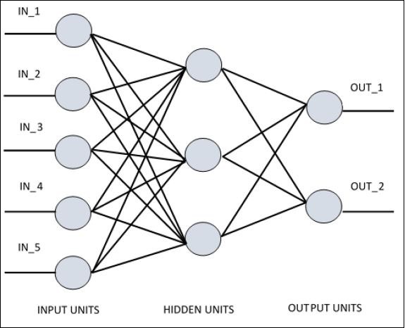
該圖顯示隱藏單元與外部層通訊。而輸入和輸出單元僅透過網路的隱藏層進行通訊。

節點的連線模式、層的總數和輸入與輸出之間節點的級別以及每層的神經元數量定義了神經網路的架構。

有兩種架構型別。這些型別關注人工神經網路的功能如下：

• 單層感知器
• 多層感知器

單層感知器

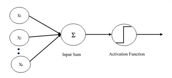
單層感知器是第一個提出的神經模型。神經元的區域性儲存器的內容包含一個權重向量。單層感知器的計算是透過計算輸入向量的總和來執行的，每個輸入向量都乘以權重向量的對應元素。輸出中顯示的值將成為啟用函式的輸入。

讓我們關注使用 TensorFlow 對影像分類問題實現單層感知器。透過“邏輯迴歸”的表示來說明單層感知器的最佳示例。

現在，讓我們考慮訓練邏輯迴歸的以下基本步驟：

• 在訓練開始時，權重用隨機值初始化。

• 對於訓練集的每個元素，使用期望輸出與實際輸出之間的差值計算誤差。計算出的誤差用於調整權重。

• 重複此過程，直到整個訓練集的誤差小於指定的閾值，或者達到最大迭代次數。

下面提到了用於評估邏輯迴歸的完整程式碼：

# Import MINST data 
from tensorflow.examples.tutorials.mnist import input_data 
mnist = input_data.read_data_sets("/tmp/data/", one_hot = True) 

import tensorflow as tf 
import matplotlib.pyplot as plt 

# Parameters 
learning_rate = 0.01 
training_epochs = 25 
batch_size = 100 
display_step = 1 

# tf Graph Input 
x = tf.placeholder("float", [None, 784]) # mnist data image of shape 28*28 = 784 
y = tf.placeholder("float", [None, 10]) # 0-9 digits recognition => 10 classes 

# Create model 
# Set model weights 
W = tf.Variable(tf.zeros([784, 10])) 
b = tf.Variable(tf.zeros([10])) 

# Construct model 
activation = tf.nn.softmax(tf.matmul(x, W) + b) # Softmax 

# Minimize error using cross entropy 
cross_entropy = y*tf.log(activation) 
cost = tf.reduce_mean\ (-tf.reduce_sum\ (cross_entropy,reduction_indices = 1)) 

optimizer = tf.train.\ GradientDescentOptimizer(learning_rate).minimize(cost) 

#Plot settings 
avg_set = [] 
epoch_set = [] 

# Initializing the variables init = tf.initialize_all_variables()
# Launch the graph 
with tf.Session() as sess:
   sess.run(init)
   
   # Training cycle
   for epoch in range(training_epochs):
      avg_cost = 0.
      total_batch = int(mnist.train.num_examples/batch_size)
      
      # Loop over all batches
      for i in range(total_batch):
         batch_xs, batch_ys = \ mnist.train.next_batch(batch_size)
         # Fit training using batch data sess.run(optimizer, \ feed_dict = {
            x: batch_xs, y: batch_ys}) 
         # Compute average loss avg_cost += sess.run(cost, \ feed_dict = {
            x: batch_xs, \ y: batch_ys})/total_batch
      # Display logs per epoch step
      if epoch % display_step == 0:
         print ("Epoch:", '%04d' % (epoch+1), "cost=", "{:.9f}".format(avg_cost))
            avg_set.append(avg_cost) epoch_set.append(epoch+1)
   print ("Training phase finished")
    
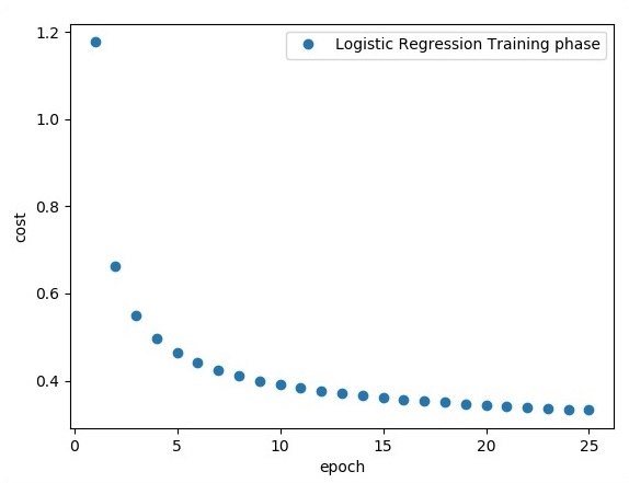
   plt.plot(epoch_set,avg_set, 'o', label = 'Logistic Regression Training phase') 
   plt.ylabel('cost') 
   plt.xlabel('epoch') 
   plt.legend() 
   plt.show() 
    
   # Test model 
   correct_prediction = tf.equal(tf.argmax(activation, 1), tf.argmax(y, 1)) 
   
   # Calculate accuracy 
   accuracy = tf.reduce_mean(tf.cast(correct_prediction, "float")) print 
      ("Model accuracy:", accuracy.eval({x: mnist.test.images, y: mnist.test.labels}))

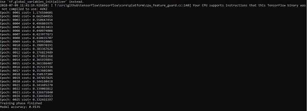
輸出

以上程式碼生成以下輸出：

邏輯迴歸被認為是一種預測分析。邏輯迴歸用於描述資料並解釋一個依賴的二元變數與一個或多個名義或自變數之間的關係。