TensorFlow - 迴圈神經網路

迴圈神經網路是一種面向深度學習的演算法，它遵循順序方法。在神經網路中，我們總是假設每個輸入和輸出都獨立於所有其他層。這些型別的神經網路被稱為迴圈神經網路，因為它們以順序方式執行數學計算。

考慮以下訓練迴圈神經網路的步驟：

步驟 1 - 從資料集中輸入一個特定的示例。

步驟 2 - 網路將獲取一個示例並使用隨機初始化的變數進行一些計算。

步驟 3 - 然後計算預測結果。

步驟 4 - 生成的實際結果與預期值的比較將產生誤差。

步驟 5 - 為了追蹤誤差，它會透過相同的路徑傳播，其中變數也會被調整。

步驟 6 - 重複步驟 1 到 5，直到我們確信宣告以獲取輸出的變數已正確定義。

步驟 7 - 透過應用這些變數來獲取新的未見輸入，從而進行系統預測。

下面描述了表示迴圈神經網路的示意圖方法：

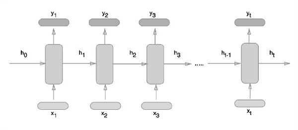
使用 TensorFlow 實現迴圈神經網路

在本節中，我們將學習如何使用 TensorFlow 實現迴圈神經網路。

步驟 1 - TensorFlow 包含用於迴圈神經網路模組的特定實現的各種庫。

#Import necessary modules
from __future__ import print_function

import tensorflow as tf
from tensorflow.contrib import rnn
from tensorflow.examples.tutorials.mnist import input_data
mnist = input_data.read_data_sets("/tmp/data/", one_hot = True)

如上所述，這些庫有助於定義輸入資料，這是迴圈神經網路實現的主要部分。

步驟 2 - 我們的主要目的是使用迴圈神經網路對影像進行分類，其中我們將每個影像行視為畫素序列。MNIST 影像形狀被專門定義為 28*28 px。現在我們將處理每個樣本的 28 個 28 步序列。我們將定義輸入引數以完成順序模式。

n_input = 28 # MNIST data input with img shape 28*28
n_steps = 28
n_hidden = 128
n_classes = 10

# tf Graph input
x = tf.placeholder("float", [None, n_steps, n_input])
y = tf.placeholder("float", [None, n_classes]
weights = {
   'out': tf.Variable(tf.random_normal([n_hidden, n_classes]))
}
biases = {
   'out': tf.Variable(tf.random_normal([n_classes]))
}

步驟 3 - 使用 RNN 中定義的函式計算結果以獲得最佳結果。在這裡，每個資料形狀都與當前輸入形狀進行比較，並計算結果以保持準確率。

def RNN(x, weights, biases):
   x = tf.unstack(x, n_steps, 1)

   # Define a lstm cell with tensorflow
   lstm_cell = rnn.BasicLSTMCell(n_hidden, forget_bias=1.0)

   # Get lstm cell output
   outputs, states = rnn.static_rnn(lstm_cell, x, dtype = tf.float32)

   # Linear activation, using rnn inner loop last output
   return tf.matmul(outputs[-1], weights['out']) + biases['out']

pred = RNN(x, weights, biases)

# Define loss and optimizer
cost = tf.reduce_mean(tf.nn.softmax_cross_entropy_with_logits(logits = pred, labels = y))
optimizer = tf.train.AdamOptimizer(learning_rate = learning_rate).minimize(cost)

# Evaluate model
correct_pred = tf.equal(tf.argmax(pred,1), tf.argmax(y,1))
accuracy = tf.reduce_mean(tf.cast(correct_pred, tf.float32))

# Initializing the variables
init = tf.global_variables_initializer()

步驟 4 - 在此步驟中，我們將啟動圖形以獲取計算結果。這也有助於計算測試結果的準確性。

with tf.Session() as sess:
   sess.run(init)
   step = 1
   # Keep training until reach max iterations
   
   while step * batch_size < training_iters:
      batch_x, batch_y = mnist.train.next_batch(batch_size)
      batch_x = batch_x.reshape((batch_size, n_steps, n_input))
      sess.run(optimizer, feed_dict={x: batch_x, y: batch_y})
      
      if step % display_step == 0:
         # Calculate batch accuracy
         acc = sess.run(accuracy, feed_dict={x: batch_x, y: batch_y})
         
         # Calculate batch loss
         loss = sess.run(cost, feed_dict={x: batch_x, y: batch_y})
         
         print("Iter " + str(step*batch_size) + ", Minibatch Loss= " + \
            "{:.6f}".format(loss) + ", Training Accuracy= " + \
            "{:.5f}".format(acc))
      step += 1
   print("Optimization Finished!")
      test_len = 128
   test_data = mnist.test.images[:test_len].reshape((-1, n_steps, n_input))
   
   test_label = mnist.test.labels[:test_len]
   print("Testing Accuracy:", \
      sess.run(accuracy, feed_dict={x: test_data, y: test_label}))

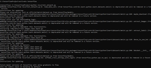
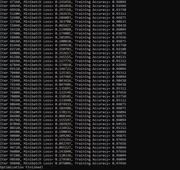
下面的螢幕截圖顯示了生成的輸出：