TensorFlow - 卷積神經網路

---

---

在理解機器學習概念之後，我們現在可以將重點轉向深度學習概念。深度學習是機器學習的一個分支，被認為是近幾十年來研究人員取得的一個關鍵步驟。深度學習實現的例子包括影像識別和語音識別等應用。

以下是兩種重要的深度神經網路型別：

• 卷積神經網路
• 迴圈神經網路

在本章中，我們將重點介紹卷積神經網路 (CNN)。

卷積神經網路

卷積神經網路旨在透過多層陣列處理資料。這種型別的神經網路用於影像識別或人臉識別等應用。CNN 與任何其他普通神經網路的主要區別在於，CNN 將輸入作為二維陣列，並直接對影像進行操作，而不是像其他神經網路那樣關注特徵提取。

CNN 的主要方法包括針對識別問題的解決方案。谷歌和Facebook 等頂級公司已投資於識別專案的研發，以更快地完成活動。

卷積神經網路使用三個基本思想：

• 區域性感受野
• 卷積
• 池化

讓我們詳細瞭解這些思想。

CNN 利用輸入資料中存在的空間相關性。神經網路的每一層都連線一些輸入神經元。這個特定區域稱為區域性感受野。區域性感受野關注隱藏神經元。隱藏神經元處理上述區域內的輸入資料，而不會意識到特定邊界外的變化。

以下是生成區域性感受野的示意圖：

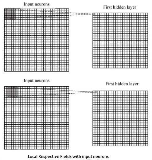
如果我們觀察上面的表示，每個連線都會學習隱藏神經元與其相關的連線的權重，並從一層移動到另一層。在這裡，單個神經元會不時地發生轉移。這個過程稱為“卷積”。

從輸入層到隱藏特徵圖的連線對映定義為“共享權重”，包含的偏差稱為“共享偏差”。

CNN 或卷積神經網路使用池化層，這些層位於 CNN 宣告之後。它將使用者的輸入作為來自卷積網路的特徵圖，並準備一個壓縮的特徵圖。池化層有助於建立具有先前層神經元的層。

TensorFlow 中 CNN 的實現

在本節中，我們將學習 CNN 的 TensorFlow 實現。執行和正確確定整個網路維度所需的步驟如下所示：

步驟 1 - 包含 TensorFlow 和資料集合模組所需的必要模組，這些模組需要計算 CNN 模型。

import tensorflow as tf
import numpy as np
from tensorflow.examples.tutorials.mnist import input_data

步驟 2 - 宣告一個名為 run_cnn() 的函式，其中包括各種引數和最佳化變數以及資料佔位符的宣告。這些最佳化變數將宣告訓練模式。

def run_cnn():
   mnist = input_data.read_data_sets("MNIST_data/", one_hot = True)
   learning_rate = 0.0001
   epochs = 10
   batch_size = 50

步驟 3 - 在此步驟中，我們將宣告訓練資料佔位符以及輸入引數 - 對於 28 x 28 畫素 = 784。這是從 mnist.train.nextbatch() 中提取的展平的影像資料。

我們可以根據需要重新調整張量的形狀。第一個值 (-1) 告訴函式根據傳遞給它的資料量動態地塑造該維度。兩個中間維度設定為影像大小（即 28 x 28）。

x = tf.placeholder(tf.float32, [None, 784])
x_shaped = tf.reshape(x, [-1, 28, 28, 1])
y = tf.placeholder(tf.float32, [None, 10])

步驟 4 - 現在重要的是建立一些卷積層：

layer1 = create_new_conv_layer(x_shaped, 1, 32, [5, 5], [2, 2], name = 'layer1')
layer2 = create_new_conv_layer(layer1, 32, 64, [5, 5], [2, 2], name = 'layer2')

步驟 5 - 讓我們展平輸出，準備用於全連線輸出階段 - 在兩層步長為 2 的池化之後，維度為 28 x 28，降為 14 x 14 或最小 7 x 7 x,y 座標，但具有 64 個輸出通道。要使用“密集”層建立全連線層，新的形狀需要是 [-1, 7 x 7 x 64]。我們可以為此層設定一些權重和偏差值，然後使用 ReLU 啟用。

flattened = tf.reshape(layer2, [-1, 7 * 7 * 64])

wd1 = tf.Variable(tf.truncated_normal([7 * 7 * 64, 1000], stddev = 0.03), name = 'wd1')
bd1 = tf.Variable(tf.truncated_normal([1000], stddev = 0.01), name = 'bd1')

dense_layer1 = tf.matmul(flattened, wd1) + bd1
dense_layer1 = tf.nn.relu(dense_layer1)

步驟 6 - 另一個具有特定 softmax 啟用函式和所需最佳化器的層定義了精度評估，這使得初始化運算子的設定成為可能。

wd2 = tf.Variable(tf.truncated_normal([1000, 10], stddev = 0.03), name = 'wd2')
bd2 = tf.Variable(tf.truncated_normal([10], stddev = 0.01), name = 'bd2')

dense_layer2 = tf.matmul(dense_layer1, wd2) + bd2
y_ = tf.nn.softmax(dense_layer2)

cross_entropy = tf.reduce_mean(
   tf.nn.softmax_cross_entropy_with_logits(logits = dense_layer2, labels = y))

optimiser = tf.train.AdamOptimizer(learning_rate = learning_rate).minimize(cross_entropy)

correct_prediction = tf.equal(tf.argmax(y, 1), tf.argmax(y_, 1))
accuracy = tf.reduce_mean(tf.cast(correct_prediction, tf.float32))

init_op = tf.global_variables_initializer()

步驟 7 - 我們應該設定記錄變數。這會新增一個摘要來儲存資料的精度。

tf.summary.scalar('accuracy', accuracy)
   merged = tf.summary.merge_all()
   writer = tf.summary.FileWriter('E:\TensorFlowProject')
   
   with tf.Session() as sess:
      sess.run(init_op)
      total_batch = int(len(mnist.train.labels) / batch_size)
      
      for epoch in range(epochs):
         avg_cost = 0
      for i in range(total_batch):
         batch_x, batch_y = mnist.train.next_batch(batch_size = batch_size)
            _, c = sess.run([optimiser, cross_entropy], feed_dict = {
            x:batch_x, y: batch_y})
            avg_cost += c / total_batch
         test_acc = sess.run(accuracy, feed_dict = {x: mnist.test.images, y:
            mnist.test.labels})
            summary = sess.run(merged, feed_dict = {x: mnist.test.images, y:
            mnist.test.labels})
         writer.add_summary(summary, epoch)

   print("\nTraining complete!")
   writer.add_graph(sess.graph)
   print(sess.run(accuracy, feed_dict = {x: mnist.test.images, y:
      mnist.test.labels}))

def create_new_conv_layer(
   input_data, num_input_channels, num_filters,filter_shape, pool_shape, name):

   conv_filt_shape = [
      filter_shape[0], filter_shape[1], num_input_channels, num_filters]

   weights = tf.Variable(
      tf.truncated_normal(conv_filt_shape, stddev = 0.03), name = name+'_W')
   bias = tf.Variable(tf.truncated_normal([num_filters]), name = name+'_b')

#Out layer defines the output
   out_layer =
      tf.nn.conv2d(input_data, weights, [1, 1, 1, 1], padding = 'SAME')

   out_layer += bias
   out_layer = tf.nn.relu(out_layer)
   ksize = [1, pool_shape[0], pool_shape[1], 1]
   strides = [1, 2, 2, 1]
   out_layer = tf.nn.max_pool(
      out_layer, ksize = ksize, strides = strides, padding = 'SAME')

   return out_layer

if __name__ == "__main__":
run_cnn()

以下是上述程式碼生成的輸出：

See @{tf.nn.softmax_cross_entropy_with_logits_v2}.

2018-09-19 17:22:58.802268: I
T:\src\github\tensorflow\tensorflow\core\platform\cpu_feature_guard.cc:140]
Your CPU supports instructions that this TensorFlow binary was not compiled to
use: AVX2

2018-09-19 17:25:41.522845: W
T:\src\github\tensorflow\tensorflow\core\framework\allocator.cc:101] Allocation
of 1003520000 exceeds 10% of system memory.

2018-09-19 17:25:44.630941: W
T:\src\github\tensorflow\tensorflow\core\framework\allocator.cc:101] Allocation
of 501760000 exceeds 10% of system memory.

Epoch: 1 cost = 0.676 test accuracy: 0.940

2018-09-19 17:26:51.987554: W
T:\src\github\tensorflow\tensorflow\core\framework\allocator.cc:101] Allocation
of 1003520000 exceeds 10% of system memory.