R - 時間序列分析

時間序列是一系列資料點，其中每個資料點都與一個時間戳相關聯。一個簡單的例子是股票市場中某隻股票在給定日期的不同時間點的價格。另一個例子是某一地區不同月份的降雨量。R 語言使用許多函式來建立、操作和繪製時間序列資料。時間序列的資料儲存在一個名為時間序列物件的 R 物件中。它也是一個 R 資料物件，如向量或資料框。

時間序列物件是使用ts()函式建立的。

語法

時間序列分析中ts()函式的基本語法如下：

timeseries.object.name <-  ts(data, start, end, frequency)

以下是所用引數的描述：

data 是一個包含時間序列中使用的值的向量或矩陣。
start 指定時間序列中第一個觀測值開始時間。
end 指定時間序列中最後一個觀測值結束時間。
frequency 指定每個時間單位的觀測次數。

除“data”引數外，所有其他引數都是可選的。

示例

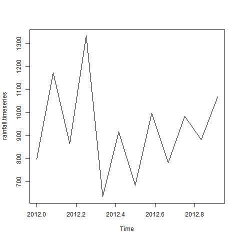
考慮從 2012 年 1 月開始某地的年降雨量詳情。我們為 12 個月建立一個 R 時間序列物件並將其繪製出來。

即時演示

# Get the data points in form of a R vector.
rainfall <- c(799,1174.8,865.1,1334.6,635.4,918.5,685.5,998.6,784.2,985,882.8,1071)

# Convert it to a time series object.
rainfall.timeseries <- ts(rainfall,start = c(2012,1),frequency = 12)

# Print the timeseries data.
print(rainfall.timeseries)

# Give the chart file a name.
png(file = "rainfall.png")

# Plot a graph of the time series.
plot(rainfall.timeseries)

# Save the file.
dev.off()

當我們執行上述程式碼時，它會產生以下結果和圖表：

Jan    Feb    Mar    Apr    May     Jun    Jul    Aug    Sep
2012  799.0  1174.8  865.1  1334.6  635.4  918.5  685.5  998.6  784.2
        Oct    Nov    Dec
2012  985.0  882.8 1071.0

時間序列圖表：

不同的時間間隔

ts() 函式中frequency引數的值決定了測量資料點的間隔。值 12 表示時間序列為 12 個月。其他值及其含義如下：

frequency = 12 將資料點固定在每年的每個月。
frequency = 4 將資料點固定在每年的每個季度。
frequency = 6 將資料點固定在每小時的每 10 分鐘。
frequency = 24*6 將資料點固定在每天的每 10 分鐘。

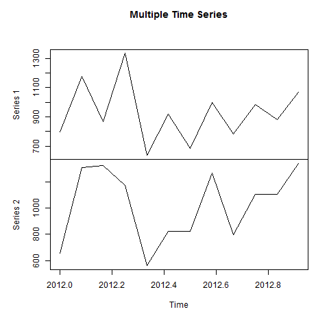
多個時間序列

我們可以透過將兩個序列組合成一個矩陣，在一個圖表中繪製多個時間序列。

即時演示

# Get the data points in form of a R vector.
rainfall1 <- c(799,1174.8,865.1,1334.6,635.4,918.5,685.5,998.6,784.2,985,882.8,1071)
rainfall2 <- 
           c(655,1306.9,1323.4,1172.2,562.2,824,822.4,1265.5,799.6,1105.6,1106.7,1337.8)

# Convert them to a matrix.
combined.rainfall <-  matrix(c(rainfall1,rainfall2),nrow = 12)

# Convert it to a time series object.
rainfall.timeseries <- ts(combined.rainfall,start = c(2012,1),frequency = 12)

# Print the timeseries data.
print(rainfall.timeseries)

# Give the chart file a name.
png(file = "rainfall_combined.png")

# Plot a graph of the time series.
plot(rainfall.timeseries, main = "Multiple Time Series")

# Save the file.
dev.off()

當我們執行上述程式碼時，它會產生以下結果和圖表：

           Series 1  Series 2
Jan 2012    799.0    655.0
Feb 2012   1174.8   1306.9
Mar 2012    865.1   1323.4
Apr 2012   1334.6   1172.2
May 2012    635.4    562.2
Jun 2012    918.5    824.0
Jul 2012    685.5    822.4
Aug 2012    998.6   1265.5
Sep 2012    784.2    799.6
Oct 2012    985.0   1105.6
Nov 2012    882.8   1106.7
Dec 2012   1071.0   1337.8

多個時間序列圖表：

列印頁面