R - 非線性最小二乘

在為迴歸分析建模真實世界資料時，我們觀察到模型的方程很少是產生線性圖表的線性方程。大多數情況下，真實世界資料的模型方程涉及較高次冪的數學函式，如 3 次冪或正弦函式。在這樣的場景中，模型的圖給出的是曲線而不是直線。線性迴歸和非線性迴歸的目標都是調整模型引數的值，以找到最接近您資料的直線或曲線。在找到這些值後，我們將能夠非常準確地估計響應變數。

在最小二乘迴歸中，我們建立一個迴歸模型，其中不同點到迴歸曲線的垂直距離的平方和最小。我們通常從一個已定義的模型開始，並假設一些係數的值。然後，我們應用 R 的 nls() 函式來獲取更準確的值以及置信區間。

語法

在 R 中建立非線性最小二乘檢驗的基本語法為 −

nls(formula, data, start)

以下是所用引數的描述 −

• formula 是包括變數和引數的非線性模型公式。

• data 是用於評估公式中變數的資料框。

• start 是起始估計值的命名列表或命名的數字向量。

示例

我們將考慮一個非線性模型，並假設其係數的初始值。接下來，我們將檢視這些假定值的置信區間，以便判斷這些值在模型中擬合得如何。

因此，讓我們為此考慮以下方程 −

a = b1*x^2+b2

我們假設初始係數為 1 和 3，並將這些值代入 nls() 函式。

xvalues <- c(1.6,2.1,2,2.23,3.71,3.25,3.4,3.86,1.19,2.21)
yvalues <- c(5.19,7.43,6.94,8.11,18.75,14.88,16.06,19.12,3.21,7.58)

# Give the chart file a name.
png(file = "nls.png")


# Plot these values.
plot(xvalues,yvalues)


# Take the assumed values and fit into the model.
model <- nls(yvalues ~ b1*xvalues^2+b2,start = list(b1 = 1,b2 = 3))

# Plot the chart with new data by fitting it to a prediction from 100 data points.
new.data <- data.frame(xvalues = seq(min(xvalues),max(xvalues),len = 100))
lines(new.data$xvalues,predict(model,newdata = new.data))

# Save the file.
dev.off()

# Get the sum of the squared residuals.
print(sum(resid(model)^2))

# Get the confidence intervals on the chosen values of the coefficients.
print(confint(model))

當我們執行上述程式碼時，它產生以下結果 −

[1] 1.081935
Waiting for profiling to be done...
       2.5%    97.5%
b1 1.137708 1.253135
b2 1.497364 2.496484

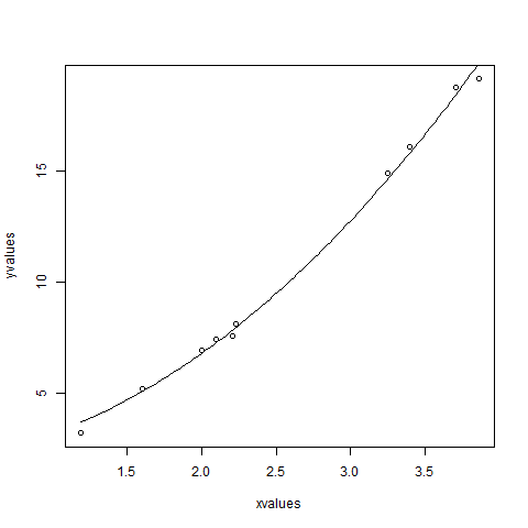
我們可以得出結論：b1 的值更接近 1，而 b2 的值更接近 2，而不是 3。