- R 教程
- R - 首頁
- R - 概述
- R - 環境設定
- R - 基本語法
- R - 資料型別
- R - 變數
- R - 運算子
- R - 決策
- R - 迴圈
- R - 函式
- R - 字串
- R - 向量
- R - 列表
- R - 矩陣
- R - 陣列
- R - 因子
- R - 資料框
- R - 包
- R - 資料重塑
R - 快速指南
R - 概述
R 是一種用於統計分析、圖形表示和報告的程式語言和軟體環境。R 由紐西蘭奧克蘭大學的 Ross Ihaka 和 Robert Gentleman 建立,目前由 R 開發核心團隊開發。
R 的核心是一種解釋型計算機語言,它允許分支和迴圈,以及使用函式進行模組化程式設計。為了提高效率,R 允許與用 C、C++、.Net、Python 或 FORTRAN 語言編寫的過程整合。
R 在 GNU 通用公共許可證下免費提供,並且為各種作業系統(如 Linux、Windows 和 Mac)提供了預編譯的二進位制版本。
R 是在 GNU 風格的版權宣告下分發的自由軟體,並且是稱為GNU S的 GNU 專案的正式組成部分。
R 的發展歷程
R 最初由紐西蘭奧克蘭大學統計系Ross Ihaka和Robert Gentleman編寫。R 於 1993 年首次出現。
一大批個人透過傳送程式碼和錯誤報告為 R 做出了貢獻。
自 1997 年年中以來,一直有一個核心小組(“R 核心團隊”)可以修改 R 原始碼檔案。
R 的特點
如前所述,R 是一種用於統計分析、圖形表示和報告的程式語言和軟體環境。以下是 R 的重要特性:
R 是一種完善的、簡單有效的程式語言,包括條件語句、迴圈語句、使用者定義的遞迴函式以及輸入輸出功能。
R 具有有效的資料處理和儲存功能。
R 提供了一套用於對陣列、列表、向量和矩陣進行計算的運算子。
R 提供了大量連貫且整合的用於資料分析的工具。
R 提供了用於資料分析和顯示的圖形功能,可以直接在計算機上顯示或列印到紙張上。
總之,R 是世界上使用最廣泛的統計程式語言。它是資料科學家的首選,並得到一個充滿活力且才華橫溢的貢獻者社群的支援。R 在大學中教授,並部署在關鍵業務應用程式中。本教程將透過簡單易懂的步驟,結合合適的示例,教你學習 R 程式設計。
R - 環境設定
本地環境設定
如果你仍然希望為 R 設定你的環境,你可以按照以下步驟操作。
Windows 安裝
你可以從R-3.2.2 for Windows (32/64 bit)下載 R 的 Windows 安裝程式版本,並將其儲存到本地目錄中。
因為它是一個名為“R-version-win.exe”的 Windows 安裝程式 (.exe)。你可以雙擊並執行安裝程式,接受預設設定。如果你的 Windows 是 32 位版本,它將安裝 32 位版本。但如果你的 Windows 是 64 位版本,則它將安裝 32 位和 64 位版本。
安裝後,你可以在 Windows 程式檔案下的“R\R3.2.2\bin\i386\Rgui.exe”目錄結構中找到執行程式的圖示。單擊此圖示將顯示 R-GUI,它是用於執行 R 程式設計的 R 控制檯。
Linux 安裝
R 可作為許多 Linux 版本的二進位制檔案,位於R 二進位制檔案。
安裝 Linux 的說明因發行版而異。這些步驟在上述連結中每個型別的 Linux 版本下都有說明。但是,如果你很著急,可以使用yum命令安裝 R,如下所示:
$ yum install R
以上命令將安裝 R 程式設計的核心功能以及標準包,如果你仍然需要其他包,則可以啟動 R 提示符,如下所示:
$ R
R version 3.2.0 (2015-04-16) -- "Full of  Ingredients"
Copyright (C) 2015 The R Foundation for Statistical Computing
Platform: x86_64-redhat-linux-gnu (64-bit)

R is free software and comes with ABSOLUTELY NO WARRANTY.
You are welcome to redistribute it under certain conditions.
Type 'license()' or 'licence()' for distribution details.

R is a collaborative project with many  contributors.
Type 'contributors()' for more information and
'citation()' on how to cite R or R packages in publications.

Type 'demo()' for some demos, 'help()' for on-line help, or
'help.start()' for an HTML browser interface to help.
Type 'q()' to quit R.
>
現在,你可以在 R 提示符下使用 install 命令安裝所需的包。例如,以下命令將安裝plotrix包,該包是 3D 圖表所需的。
> install.packages("plotrix")
R - 基本語法
按照慣例,我們將透過編寫一個“Hello, World!”程式開始學習 R 程式設計。根據需要,你可以在 R 命令提示符下程式設計,也可以使用 R 指令碼檔案編寫程式。讓我們逐一檢查兩者。
R 命令提示符
一旦你設定了 R 環境,只需在你的命令提示符下鍵入以下命令即可輕鬆啟動 R 命令提示符:
$ R
這將啟動 R 直譯器,你將獲得一個提示符>,你可以在其中開始鍵入程式,如下所示:
> myString <- "Hello, World!"
> print ( myString)
[1] "Hello, World!"
這裡第一條語句定義了一個字串變數 myString,我們為其賦值一個字串“Hello, World!”,然後下一條語句 print() 用於列印儲存在變數 myString 中的值。
R 指令碼檔案
通常,你將透過在指令碼檔案中編寫程式來進行程式設計,然後在命令提示符下使用稱為Rscript的 R 直譯器執行這些指令碼。因此,讓我們從在名為 test.R 的文字檔案中編寫以下程式碼開始:
# My first program in R Programming
myString <- "Hello, World!"

print ( myString)
將以上程式碼儲存到檔案 test.R 中,並在 Linux 命令提示符下執行,如下所示。即使你使用 Windows 或其他系統,語法也將保持不變。
$ Rscript test.R
當我們執行以上程式時,它會產生以下結果。
[1] "Hello, World!"
註釋
註釋就像 R 程式中的幫助文字,在執行實際程式時,直譯器會忽略它們。單行註釋使用#作為語句的開頭,如下所示:
# My first program in R Programming
R 不支援多行註釋,但你可以使用一種技巧,如下所示:
if(FALSE) {
   "This is a demo for multi-line comments and it should be put inside either a
      single OR double quote"
}

myString <- "Hello, World!"
print ( myString)
[1] "Hello, World!"
雖然以上註釋將由 R 直譯器執行,但它們不會干擾你的實際程式。你應該將此類註釋放在單引號或雙引號內。
R - 資料型別
通常,在任何程式語言中進行程式設計時,都需要使用各種變數來儲存各種資訊。變數只不過是保留的記憶體位置,用於儲存值。這意味著,當你建立變數時,會在記憶體中保留一些空間。
你可能希望儲存各種資料型別的資訊,如字元、寬字元、整數、浮點數、雙精度浮點數、布林值等。根據變數的資料型別,作業系統會分配記憶體並決定在保留的記憶體中可以儲存什麼。
與其他程式語言(如 C 和 Java)不同,在 R 中,變數不會被宣告為某種資料型別。變數被賦予 R 物件,R 物件的資料型別成為變數的資料型別。R 物件有很多型別。常用的有:
- 向量
- 列表
- 矩陣
- 陣列
- 因子
- 資料框
其中最簡單的物件是向量物件,這些原子向量有六種資料型別,也稱為六類向量。其他 R 物件是建立在原子向量之上的。
| 資料型別 | 示例 | 驗證 |
|---|---|---|
| 邏輯型 | TRUE, FALSE |
v <- TRUE
print(class(v))
它會產生以下結果: [1] "logical" |
| 數值型 | 12.3, 5, 999 |
v <- 23.5
print(class(v))
它會產生以下結果: [1] "numeric" |
| 整數型 | 2L, 34L, 0L |
v <- 2L
print(class(v))
它會產生以下結果: [1] "integer" |
| 複數型 | 3 + 2i |
v <- 2+5i
print(class(v))
它會產生以下結果: [1] "complex" |
| 字元型 | 'a' , '"good", "TRUE", '23.4' |
v <- "TRUE"
print(class(v))
它會產生以下結果: [1] "character" |
| 原始型 | "Hello" 儲存為 48 65 6c 6c 6f |
v <- charToRaw("Hello")
print(class(v))
它會產生以下結果: [1] "raw" |
在 R 程式設計中,最基本的資料型別是稱為向量的 R 物件,它可以儲存不同類別的元素,如上所示。請注意,在 R 中,類別的數量不僅限於以上六種型別。例如,我們可以使用許多原子向量並建立一個數組,其類別將成為陣列。
向量
當你想建立一個包含多個元素的向量時,應該使用c()函式,它表示將元素組合成一個向量。
# Create a vector.
apple <- c('red','green',"yellow")
print(apple)

# Get the class of the vector.
print(class(apple))
當我們執行以上程式碼時,它會產生以下結果:
[1] "red"    "green"  "yellow"
[1] "character"
列表
列表是 R 物件,它可以在其中包含許多不同型別的元素,如向量、函式甚至另一個列表。
# Create a list.
list1 <- list(c(2,5,3),21.3,sin)

# Print the list.
print(list1)
當我們執行以上程式碼時,它會產生以下結果:
[[1]]
[1] 2 5 3

[[2]]
[1] 21.3

[[3]]
function (x)  .Primitive("sin")
矩陣
矩陣是一個二維的矩形資料集。它可以使用向量輸入到矩陣函式中建立。
# Create a matrix.
M = matrix( c('a','a','b','c','b','a'), nrow = 2, ncol = 3, byrow = TRUE)
print(M)
當我們執行以上程式碼時,它會產生以下結果:
     [,1] [,2] [,3]
[1,] "a"  "a"  "b"
[2,] "c"  "b"  "a"
陣列
雖然矩陣僅限於兩個維度,但陣列可以是任意數量的維度。array 函式採用一個 dim 屬性,該屬性建立所需的維度數。在下面的示例中,我們建立了一個包含兩個元素的陣列,每個元素都是一個 3x3 矩陣。
# Create an array.
a <- array(c('green','yellow'),dim = c(3,3,2))
print(a)
當我們執行以上程式碼時,它會產生以下結果:
, , 1

     [,1]     [,2]     [,3]
[1,] "green"  "yellow" "green"
[2,] "yellow" "green"  "yellow"
[3,] "green"  "yellow" "green"

, , 2

     [,1]     [,2]     [,3]
[1,] "yellow" "green"  "yellow"
[2,] "green"  "yellow" "green"
[3,] "yellow" "green"  "yellow"
因子
因子是使用向量建立的 r 物件。它儲存向量以及向量中元素的不同值作為標籤。無論輸入向量是數值型、字元型還是布林型等,標籤始終為字元型。它們在統計建模中很有用。
因子使用factor()函式建立。nlevels函式給出級別的數量。
# Create a vector.
apple_colors <- c('green','green','yellow','red','red','red','green')

# Create a factor object.
factor_apple <- factor(apple_colors)

# Print the factor.
print(factor_apple)
print(nlevels(factor_apple))
當我們執行以上程式碼時,它會產生以下結果:
[1] green  green  yellow red    red    red    green
Levels: green red yellow
[1] 3
資料框
資料框是表格資料物件。與矩陣不同,在資料框中,每一列可以包含不同的資料模式。第一列可以是數值型,而第二列可以是字元型,第三列可以是邏輯型。它是一個長度相等的向量的列表。
資料框使用data.frame()函式建立。
# Create the data frame.
BMI <- 	data.frame(
   gender = c("Male", "Male","Female"),
   height = c(152, 171.5, 165),
   weight = c(81,93, 78),
   Age = c(42,38,26)
)
print(BMI)
當我們執行以上程式碼時,它會產生以下結果:
  gender height weight Age
1   Male  152.0     81  42
2   Male  171.5     93  38
3 Female  165.0     78  26
R - 變數
變數為我們的程式提供了可操作的命名儲存。R中的變數可以儲存原子向量、原子向量的組或許多R物件的組合。有效的變數名由字母、數字以及點或下劃線字元組成。變數名以字母或點開頭,後面不跟著數字。
| 變數名 | 有效性 | 原因 |
|---|---|---|
| var_name2. | 有效 | 包含字母、數字、點和下劃線 |
| var_name% | 無效 | 包含字元'%'。僅允許點(.)和下劃線。 |
| 2var_name | 無效 | 以數字開頭 |
.var_name, var.name |
有效 | 可以以點(.)開頭,但點(.)後面不能跟著數字。 |
| .2var_name | 無效 | 起始點後跟著數字,使其無效。 |
| _var_name | 無效 | 以_開頭,無效 |
變數賦值
可以使用左向、右向和等於運算子為變數賦值。可以使用print()或cat()函式列印變數的值。cat()函式將多個專案組合成連續的列印輸出。
# Assignment using equal operator.
var.1 = c(0,1,2,3)

# Assignment using leftward operator.
var.2 <- c("learn","R")

# Assignment using rightward operator.
c(TRUE,1) -> var.3

print(var.1)
cat ("var.1 is ", var.1 ,"\n")
cat ("var.2 is ", var.2 ,"\n")
cat ("var.3 is ", var.3 ,"\n")
當我們執行以上程式碼時,它會產生以下結果:
[1] 0 1 2 3
var.1 is  0 1 2 3
var.2 is  learn R
var.3 is  1 1
注意 - 向量c(TRUE,1)混合了邏輯和數值型別。因此邏輯型別被強制轉換為數值型別,將TRUE視為1。
變數的資料型別
在R中,變數本身沒有宣告任何資料型別,而是獲取分配給它的R物件的型別。因此R被稱為動態型別語言,這意味著我們可以在程式中使用同一個變數時,反覆更改變數的資料型別。
var_x <- "Hello"
cat("The class of var_x is ",class(var_x),"\n")

var_x <- 34.5
cat("  Now the class of var_x is ",class(var_x),"\n")

var_x <- 27L
cat("   Next the class of var_x becomes ",class(var_x),"\n")
當我們執行以上程式碼時,它會產生以下結果:
The class of var_x is  character
   Now the class of var_x is  numeric
      Next the class of var_x becomes  integer
查詢變數
要了解當前工作空間中所有可用的變數,我們使用ls()函式。此外,ls()函式可以使用模式匹配變數名。
print(ls())
當我們執行以上程式碼時,它會產生以下結果:
[1] "my var"     "my_new_var" "my_var"     "var.1"
[5] "var.2"      "var.3"      "var.name"   "var_name2."
[9] "var_x"      "varname"
注意 - 這是一個示例輸出,具體取決於您的環境中聲明瞭哪些變數。
ls()函式可以使用模式匹配變數名。
# List the variables starting with the pattern "var".
print(ls(pattern = "var"))
當我們執行以上程式碼時,它會產生以下結果:
[1] "my var"     "my_new_var" "my_var"     "var.1"
[5] "var.2"      "var.3"      "var.name"   "var_name2."
[9] "var_x"      "varname"
以點(.)開頭的變數是隱藏的,可以使用"all.names = TRUE"引數傳遞給ls()函式來列出它們。
print(ls(all.name = TRUE))
當我們執行以上程式碼時,它會產生以下結果:
[1] ".cars"        ".Random.seed" ".var_name"    ".varname"     ".varname2"
[6] "my var"       "my_new_var"   "my_var"       "var.1"        "var.2"
[11]"var.3"        "var.name"     "var_name2."   "var_x"
刪除變數
可以使用rm()函式刪除變數。下面我們刪除變數var.3。列印變數值時會丟擲錯誤。
rm(var.3)
print(var.3)
當我們執行以上程式碼時,它會產生以下結果:
[1] "var.3"
Error in print(var.3) : object 'var.3' not found
可以使用rm()和ls()函式一起刪除所有變數。
rm(list = ls())
print(ls())
當我們執行以上程式碼時,它會產生以下結果:
character(0)
R - 運算子
運算子是告訴編譯器執行特定數學或邏輯操作的符號。R語言富含內建運算子,並提供以下型別的運算子。
運算子型別
R程式設計中包含以下型別的運算子:
- 算術運算子
- 關係運算符
- 邏輯運算子
- 賦值運算子
- 其他運算子
算術運算子
下表顯示了R語言支援的算術運算子。運算子作用於向量的每個元素。
| 運算子 | 描述 | 示例 |
|---|---|---|
| + | 將兩個向量相加 |
v <- c( 2,5.5,6)
t <- c(8, 3, 4)
print(v+t)
它會產生以下結果: [1] 10.0 8.5 10.0 |
| − | 從第一個向量中減去第二個向量 |
v <- c( 2,5.5,6)
t <- c(8, 3, 4)
print(v-t)
它會產生以下結果: [1] -6.0 2.5 2.0 |
| * | 將兩個向量相乘 |
v <- c( 2,5.5,6)
t <- c(8, 3, 4)
print(v*t)
它會產生以下結果: [1] 16.0 16.5 24.0 |
| / | 將第一個向量除以第二個向量 |
v <- c( 2,5.5,6)
t <- c(8, 3, 4)
print(v/t)
當我們執行以上程式碼時,它會產生以下結果: [1] 0.250000 1.833333 1.500000 |
| %% | 第一個向量除以第二個向量的餘數 |
v <- c( 2,5.5,6)
t <- c(8, 3, 4)
print(v%%t)
它會產生以下結果: [1] 2.0 2.5 2.0 |
| %/% | 第一個向量除以第二個向量的結果(商) |
v <- c( 2,5.5,6)
t <- c(8, 3, 4)
print(v%/%t)
它會產生以下結果: [1] 0 1 1 |
| ^ | 第一個向量以第二個向量為指數的冪 |
v <- c( 2,5.5,6)
t <- c(8, 3, 4)
print(v^t)
它會產生以下結果: [1] 256.000 166.375 1296.000 |
關係運算符
下表顯示了R語言支援的關係運算符。第一個向量的每個元素都與第二個向量的對應元素進行比較。比較結果為布林值。
| 運算子 | 描述 | 示例 |
|---|---|---|
| > | 檢查第一個向量的每個元素是否大於第二個向量的對應元素。 |
v <- c(2,5.5,6,9)
t <- c(8,2.5,14,9)
print(v>t)
它會產生以下結果: [1] FALSE TRUE FALSE FALSE |
| < | 檢查第一個向量的每個元素是否小於第二個向量的對應元素。 |
v <- c(2,5.5,6,9)
t <- c(8,2.5,14,9)
print(v < t)
它會產生以下結果: [1] TRUE FALSE TRUE FALSE |
| == | 檢查第一個向量的每個元素是否等於第二個向量的對應元素。 |
v <- c(2,5.5,6,9)
t <- c(8,2.5,14,9)
print(v == t)
它會產生以下結果: [1] FALSE FALSE FALSE TRUE |
| <= | 檢查第一個向量的每個元素是否小於或等於第二個向量的對應元素。 |
v <- c(2,5.5,6,9)
t <- c(8,2.5,14,9)
print(v<=t)
它會產生以下結果: [1] TRUE FALSE TRUE TRUE |
| >= | 檢查第一個向量的每個元素是否大於或等於第二個向量的對應元素。 |
v <- c(2,5.5,6,9)
t <- c(8,2.5,14,9)
print(v>=t)
它會產生以下結果: [1] FALSE TRUE FALSE TRUE |
| != | 檢查第一個向量的每個元素是否不等於第二個向量的對應元素。 |
v <- c(2,5.5,6,9)
t <- c(8,2.5,14,9)
print(v!=t)
它會產生以下結果: [1] TRUE TRUE TRUE FALSE |
邏輯運算子
下表顯示了R語言支援的邏輯運算子。它僅適用於邏輯、數值或複數型別的向量。所有大於1的數字都被視為邏輯值TRUE。
第一個向量的每個元素都與第二個向量的對應元素進行比較。比較結果為布林值。
| 運算子 | 描述 | 示例 |
|---|---|---|
| & | 稱為逐元素邏輯與運算子。它將第一個向量的每個元素與第二個向量的對應元素組合,如果兩個元素都為TRUE,則輸出TRUE。 |
v <- c(3,1,TRUE,2+3i)
t <- c(4,1,FALSE,2+3i)
print(v&t)
它會產生以下結果: [1] TRUE TRUE FALSE TRUE |
| | | 稱為逐元素邏輯或運算子。它將第一個向量的每個元素與第二個向量的對應元素組合,如果其中一個元素為TRUE,則輸出TRUE。 |
v <- c(3,0,TRUE,2+2i)
t <- c(4,0,FALSE,2+3i)
print(v|t)
它會產生以下結果: [1] TRUE FALSE TRUE TRUE |
| ! | 稱為邏輯非運算子。獲取向量的每個元素並給出相反的邏輯值。 |
v <- c(3,0,TRUE,2+2i)
print(!v)
它會產生以下結果: [1] FALSE TRUE FALSE FALSE |
邏輯運算子&&和||僅考慮向量的第一個元素,並輸出單個元素的向量。
| 運算子 | 描述 | 示例 |
|---|---|---|
| && | 稱為邏輯與運算子。獲取兩個向量的第一個元素,並且只有當兩者都為TRUE時才輸出TRUE。 |
v <- c(3,0,TRUE,2+2i)
t <- c(1,3,TRUE,2+3i)
print(v&&t)
它會產生以下結果: [1] TRUE |
| || | 稱為邏輯或運算子。獲取兩個向量的第一個元素,如果其中一個為TRUE,則輸出TRUE。 |
v <- c(0,0,TRUE,2+2i)
t <- c(0,3,TRUE,2+3i)
print(v||t)
它會產生以下結果: [1] FALSE |
賦值運算子
這些運算子用於為向量賦值。
| 運算子 | 描述 | 示例 |
|---|---|---|
|
<− 或 = 或 <<− |
稱為左賦值 |
v1 <- c(3,1,TRUE,2+3i)
v2 <<- c(3,1,TRUE,2+3i)
v3 = c(3,1,TRUE,2+3i)
print(v1)
print(v2)
print(v3)
它會產生以下結果: [1] 3+0i 1+0i 1+0i 2+3i [1] 3+0i 1+0i 1+0i 2+3i [1] 3+0i 1+0i 1+0i 2+3i |
|
-> 或 ->> |
稱為右賦值 |
c(3,1,TRUE,2+3i) -> v1
c(3,1,TRUE,2+3i) ->> v2
print(v1)
print(v2)
它會產生以下結果: [1] 3+0i 1+0i 1+0i 2+3i [1] 3+0i 1+0i 1+0i 2+3i |
其他運算子
這些運算子用於特定目的,而不是一般的數學或邏輯計算。
| 運算子 | 描述 | 示例 |
|---|---|---|
| : | 冒號運算子。它為向量建立一系列按順序排列的數字。 |
v <- 2:8
print(v)
它會產生以下結果: [1] 2 3 4 5 6 7 8 |
| %in% | 此運算子用於識別元素是否屬於向量。 |
v1 <- 8
v2 <- 12
t <- 1:10
print(v1 %in% t)
print(v2 %in% t)
它會產生以下結果: [1] TRUE [1] FALSE |
| %*% | 此運算子用於將矩陣與其轉置相乘。 |
M = matrix( c(2,6,5,1,10,4), nrow = 2,ncol = 3,byrow = TRUE)
t = M %*% t(M)
print(t)
它會產生以下結果: [,1] [,2] [1,] 65 82 [2,] 82 117 |
R - 決策
決策結構要求程式設計師指定一個或多個條件供程式評估或測試,以及如果條件確定為true則要執行的語句,以及可選地,如果條件確定為false則要執行的其他語句。
以下是大多數程式語言中常見決策結構的一般形式:
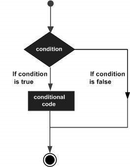
R提供以下型別的決策語句。單擊以下連結以檢視其詳細資訊。
| 序號 | 語句和描述 |
|---|---|
| 1 |
if語句
if語句由一個布林表示式後跟一個或多個語句組成。 |
| 2 |
if...else語句
if語句後可以跟一個可選的else語句,當布林表示式為false時執行。 |
| 3 |
switch語句
switch語句允許將變數與其值列表進行相等性測試。 |
R - 迴圈
可能存在需要多次執行程式碼塊的情況。通常,語句按順序執行。函式中的第一個語句首先執行,然後是第二個語句,依此類推。
程式語言提供各種控制結構,允許更復雜的執行路徑。
迴圈語句允許我們將語句或語句組執行多次,以下是在大多數程式語言中迴圈語句的一般形式:
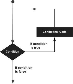
R程式語言提供以下幾種迴圈來處理迴圈需求。單擊以下連結以檢視其詳細資訊。
| 序號 | 迴圈型別和描述 |
|---|---|
| 1 |
repeat迴圈
多次執行一系列語句,並縮寫管理迴圈變數的程式碼。 |
| 2 |
while迴圈
當給定條件為true時重複語句或語句組。它在執行迴圈體之前測試條件。 |
| 3 |
for迴圈
類似於while語句,只是它在迴圈體結束時測試條件。 |
迴圈控制語句
迴圈控制語句更改執行的正常順序。當執行離開作用域時,在該作用域中建立的所有自動物件都會被銷燬。
R支援以下控制語句。單擊以下連結以檢視其詳細資訊。
R - 函式
函式是一組組織在一起以執行特定任務的語句。R有大量內建函式,使用者可以建立自己的函式。
在R中,函式是一個物件,因此R直譯器能夠將控制權傳遞給函式,以及函式完成操作可能需要的引數。
然後,函式執行其任務並將控制權以及任何可能儲存在其他物件中的結果返回給直譯器。
函式定義
R函式是使用關鍵字function建立的。R函式定義的基本語法如下:
function_name <- function(arg_1, arg_2, ...) {
   Function body
}
函式元件
函式的不同部分是:
函式名 - 這是函式的實際名稱。它作為具有此名稱的物件儲存在R環境中。
引數 - 引數是一個佔位符。當呼叫函式時,您將值傳遞給引數。引數是可選的;也就是說,函式可能不包含任何引數。引數也可以具有預設值。
函式體 - 函式體包含定義函式功能的一系列語句。
返回值 - 函式的返回值是函式體中最後一個要計算的表示式。
R有很多內建函式,可以在程式中直接呼叫,而無需先定義它們。我們還可以建立和使用我們自己的函式,稱為使用者定義函式。
內建函式
內建函式的簡單示例有seq()、mean()、max()、sum(x)和paste(...)等。它們由使用者編寫的程式直接呼叫。您可以參考最常用的R函式。
# Create a sequence of numbers from 32 to 44.
print(seq(32,44))

# Find mean of numbers from 25 to 82.
print(mean(25:82))

# Find sum of numbers frm 41 to 68.
print(sum(41:68))
當我們執行以上程式碼時,它會產生以下結果:
[1] 32 33 34 35 36 37 38 39 40 41 42 43 44
[1] 53.5
[1] 1526
使用者定義函式
我們可以在R中建立使用者定義函式。它們特定於使用者想要的功能,並且一旦建立,就可以像內建函式一樣使用。下面是一個建立和使用函式的示例。
# Create a function to print squares of numbers in sequence.
new.function <- function(a) {
   for(i in 1:a) {
      b <- i^2
      print(b)
   }
}
呼叫函式
# Create a function to print squares of numbers in sequence.
new.function <- function(a) {
   for(i in 1:a) {
      b <- i^2
      print(b)
   }
}

# Call the function new.function supplying 6 as an argument.
new.function(6)
當我們執行以上程式碼時,它會產生以下結果:
[1] 1
[1] 4
[1] 9
[1] 16
[1] 25
[1] 36
無引數呼叫函式
# Create a function without an argument.
new.function <- function() {
   for(i in 1:5) {
      print(i^2)
   }
}

# Call the function without supplying an argument.
new.function()
當我們執行以上程式碼時,它會產生以下結果:
[1] 1
[1] 4
[1] 9
[1] 16
[1] 25
帶引數值呼叫函式(按位置和按名稱)
函式呼叫的引數可以按函式中定義的相同順序提供,也可以按不同的順序提供,但分配給引數的名稱。
# Create a function with arguments.
new.function <- function(a,b,c) {
   result <- a * b + c
   print(result)
}

# Call the function by position of arguments.
new.function(5,3,11)

# Call the function by names of the arguments.
new.function(a = 11, b = 5, c = 3)
當我們執行以上程式碼時,它會產生以下結果:
[1] 26
[1] 58
使用預設引數呼叫函式
我們可以在函式定義中定義引數的值,並在呼叫函式時不提供任何引數來獲取預設結果。但是我們也可以透過提供引數的新值來呼叫此類函式並獲取非預設結果。
# Create a function with arguments.
new.function <- function(a = 3, b = 6) {
   result <- a * b
   print(result)
}

# Call the function without giving any argument.
new.function()

# Call the function with giving new values of the argument.
new.function(9,5)
當我們執行以上程式碼時,它會產生以下結果:
[1] 18
[1] 45
函式的惰性求值
函式的引數是惰性求值的,這意味著它們僅在函式體需要時才進行求值。
# Create a function with arguments.
new.function <- function(a, b) {
   print(a^2)
   print(a)
   print(b)
}

# Evaluate the function without supplying one of the arguments.
new.function(6)
當我們執行以上程式碼時,它會產生以下結果:
[1] 36
[1] 6
Error in print(b) : argument "b" is missing, with no default
R - 字串
在 R 中,任何用單引號或雙引號括起來的值都被視為字串。在內部,即使您使用單引號建立字串,R 也會將每個字串儲存在雙引號中。
字串構造規則
字串開頭和結尾的引號必須都是雙引號或都是單引號。它們不能混合使用。
雙引號可以插入到以單引號開頭和結尾的字串中。
單引號可以插入到以雙引號開頭和結尾的字串中。
雙引號不能插入到以雙引號開頭和結尾的字串中。
單引號不能插入到以單引號開頭和結尾的字串中。
有效字串示例
以下示例闡明瞭在 R 中建立字串的規則。
a <- 'Start and end with single quote'
print(a)

b <- "Start and end with double quotes"
print(b)

c <- "single quote ' in between double quotes"
print(c)

d <- 'Double quotes " in between single quote'
print(d)
執行上述程式碼後,我們將獲得以下輸出:
[1] "Start and end with single quote"
[1] "Start and end with double quotes"
[1] "single quote ' in between double quote"
[1] "Double quote \" in between single quote"
無效字串示例
e <- 'Mixed quotes"
print(e)

f <- 'Single quote ' inside single quote'
print(f)

g <- "Double quotes " inside double quotes"
print(g)
當我們執行指令碼時,它會失敗並給出以下結果。
Error: unexpected symbol in:
"print(e)
f <- 'Single"
Execution halted
字串操作
連線字串 - paste() 函式
R 中的許多字串都是使用 **paste()** 函式組合在一起的。它可以接受任意數量的引數,並將它們組合在一起。
語法
paste 函式的基本語法如下:
paste(..., sep = " ", collapse = NULL)
以下是所用引數的描述:
**...** 表示要組合的任意數量的引數。
**sep** 表示引數之間的任何分隔符。它是可選的。
**collapse** 用於消除兩個字串之間的空格。但不會消除一個字串中兩個單詞之間的空格。
示例
a <- "Hello"
b <- 'How'
c <- "are you? "

print(paste(a,b,c))

print(paste(a,b,c, sep = "-"))

print(paste(a,b,c, sep = "", collapse = ""))
當我們執行以上程式碼時,它會產生以下結果:
[1] "Hello How are you? "
[1] "Hello-How-are you? "
[1] "HelloHoware you? "
格式化數字和字串 - format() 函式
可以使用 **format()** 函式將數字和字串格式化為特定樣式。
語法
format 函式的基本語法如下:
format(x, digits, nsmall, scientific, width, justify = c("left", "right", "centre", "none"))
以下是所用引數的描述:
**x** 是向量輸入。
**digits** 是顯示的數字總數。
**nsmall** 是小數點右側的最小位數。
**scientific** 設定為 TRUE 以顯示科學計數法。
**width** 表示透過在開頭填充空格來顯示的最小寬度。
**justify** 是字串向左、向右或居中的顯示方式。
示例
# Total number of digits displayed. Last digit rounded off.
result <- format(23.123456789, digits = 9)
print(result)

# Display numbers in scientific notation.
result <- format(c(6, 13.14521), scientific = TRUE)
print(result)

# The minimum number of digits to the right of the decimal point.
result <- format(23.47, nsmall = 5)
print(result)

# Format treats everything as a string.
result <- format(6)
print(result)

# Numbers are padded with blank in the beginning for width.
result <- format(13.7, width = 6)
print(result)

# Left justify strings.
result <- format("Hello", width = 8, justify = "l")
print(result)

# Justfy string with center.
result <- format("Hello", width = 8, justify = "c")
print(result)
當我們執行以上程式碼時,它會產生以下結果:
[1] "23.1234568"
[1] "6.000000e+00" "1.314521e+01"
[1] "23.47000"
[1] "6"
[1] "  13.7"
[1] "Hello   "
[1] " Hello  "
計算字串中字元的數量 - nchar() 函式
此函式計算字串中字元的數量,包括空格。
語法
nchar() 函式的基本語法如下:
nchar(x)
以下是所用引數的描述:
**x** 是向量輸入。
示例
result <- nchar("Count the number of characters")
print(result)
當我們執行以上程式碼時,它會產生以下結果:
[1] 30
更改大小寫 - toupper() 和 tolower() 函式
這些函式更改字串字元的大小寫。
語法
toupper() 和 tolower() 函式的基本語法如下:
toupper(x)
tolower(x)
以下是所用引數的描述:
**x** 是向量輸入。
示例
# Changing to Upper case.
result <- toupper("Changing To Upper")
print(result)

# Changing to lower case.
result <- tolower("Changing To Lower")
print(result)
當我們執行以上程式碼時,它會產生以下結果:
[1] "CHANGING TO UPPER"
[1] "changing to lower"
提取字串的部分 - substring() 函式
此函式提取字串的部分。
語法
substring() 函式的基本語法如下:
substring(x,first,last)
以下是所用引數的描述:
**x** 是字元向量輸入。
**first** 是要提取的第一個字元的位置。
**last** 是要提取的最後一個字元的位置。
示例
# Extract characters from 5th to 7th position.
result <- substring("Extract", 5, 7)
print(result)
當我們執行以上程式碼時,它會產生以下結果:
[1] "act"
R - 向量
向量是 R 中最基本的資料物件,共有六種原子向量型別。它們分別是邏輯型、整型、雙精度型、複數型、字元型和原始型。
向量建立
單元素向量
即使您在 R 中只寫一個值,它也會變成長度為 1 的向量,並屬於上述向量型別之一。
# Atomic vector of type character.
print("abc");

# Atomic vector of type double.
print(12.5)

# Atomic vector of type integer.
print(63L)

# Atomic vector of type logical.
print(TRUE)

# Atomic vector of type complex.
print(2+3i)

# Atomic vector of type raw.
print(charToRaw('hello'))
當我們執行以上程式碼時,它會產生以下結果:
[1] "abc"
[1] 12.5
[1] 63
[1] TRUE
[1] 2+3i
[1] 68 65 6c 6c 6f
多元素向量
對數值資料使用冒號運算子
# Creating a sequence from 5 to 13.
v <- 5:13
print(v)

# Creating a sequence from 6.6 to 12.6.
v <- 6.6:12.6
print(v)

# If the final element specified does not belong to the sequence then it is discarded.
v <- 3.8:11.4
print(v)
當我們執行以上程式碼時,它會產生以下結果:
[1]  5  6  7  8  9 10 11 12 13
[1]  6.6  7.6  8.6  9.6 10.6 11.6 12.6
[1]  3.8  4.8  5.8  6.8  7.8  8.8  9.8 10.8
使用序列 (Seq.) 運算子
# Create vector with elements from 5 to 9 incrementing by 0.4.
print(seq(5, 9, by = 0.4))
當我們執行以上程式碼時,它會產生以下結果:
[1] 5.0 5.4 5.8 6.2 6.6 7.0 7.4 7.8 8.2 8.6 9.0
使用 c() 函式
如果元素之一是字元,則非字元值將強制轉換為字元型別。
# The logical and numeric values are converted to characters.
s <- c('apple','red',5,TRUE)
print(s)
當我們執行以上程式碼時,它會產生以下結果:
[1] "apple" "red" "5" "TRUE"
訪問向量元素
使用索引訪問向量的元素。**[ ] 方括號** 用於索引。索引從位置 1 開始。在索引中給出負值會從結果中刪除該元素。**TRUE**、**FALSE** 或 **0** 和 **1** 也可以用於索引。
# Accessing vector elements using position.
t <- c("Sun","Mon","Tue","Wed","Thurs","Fri","Sat")
u <- t[c(2,3,6)]
print(u)

# Accessing vector elements using logical indexing.
v <- t[c(TRUE,FALSE,FALSE,FALSE,FALSE,TRUE,FALSE)]
print(v)

# Accessing vector elements using negative indexing.
x <- t[c(-2,-5)]
print(x)

# Accessing vector elements using 0/1 indexing.
y <- t[c(0,0,0,0,0,0,1)]
print(y)
當我們執行以上程式碼時,它會產生以下結果:
[1] "Mon" "Tue" "Fri"
[1] "Sun" "Fri"
[1] "Sun" "Tue" "Wed" "Fri" "Sat"
[1] "Sun"
向量操作
向量算術
可以將兩個相同長度的向量相加、相減、相乘或相除,結果為向量輸出。
# Create two vectors.
v1 <- c(3,8,4,5,0,11)
v2 <- c(4,11,0,8,1,2)

# Vector addition.
add.result <- v1+v2
print(add.result)

# Vector subtraction.
sub.result <- v1-v2
print(sub.result)

# Vector multiplication.
multi.result <- v1*v2
print(multi.result)

# Vector division.
divi.result <- v1/v2
print(divi.result)
當我們執行以上程式碼時,它會產生以下結果:
[1]  7 19  4 13  1 13
[1] -1 -3  4 -3 -1  9
[1] 12 88  0 40  0 22
[1] 0.7500000 0.7272727       Inf 0.6250000 0.0000000 5.5000000
向量元素迴圈
如果我們將算術運算應用於兩個長度不相等的向量,則較短向量的元素將被迴圈使用以完成運算。
v1 <- c(3,8,4,5,0,11)
v2 <- c(4,11)
# V2 becomes c(4,11,4,11,4,11)

add.result <- v1+v2
print(add.result)

sub.result <- v1-v2
print(sub.result)
當我們執行以上程式碼時,它會產生以下結果:
[1]  7 19  8 16  4 22
[1] -1 -3  0 -6 -4  0
向量元素排序
可以使用 **sort()** 函式對向量中的元素進行排序。
v <- c(3,8,4,5,0,11, -9, 304)

# Sort the elements of the vector.
sort.result <- sort(v)
print(sort.result)

# Sort the elements in the reverse order.
revsort.result <- sort(v, decreasing = TRUE)
print(revsort.result)

# Sorting character vectors.
v <- c("Red","Blue","yellow","violet")
sort.result <- sort(v)
print(sort.result)

# Sorting character vectors in reverse order.
revsort.result <- sort(v, decreasing = TRUE)
print(revsort.result)
當我們執行以上程式碼時,它會產生以下結果:
[1]  -9   0   3   4   5   8  11 304
[1] 304  11   8   5   4   3   0  -9
[1] "Blue"   "Red"    "violet" "yellow"
[1] "yellow" "violet" "Red"    "Blue"
R - 列表
列表是 R 物件,其中包含不同型別的元素,例如:數字、字串、向量以及其內部的另一個列表。列表還可以包含矩陣或函式作為其元素。列表是使用 **list()** 函式建立的。
建立列表
以下是一個建立包含字串、數字、向量和邏輯值的列表的示例。
# Create a list containing strings, numbers, vectors and a logical
# values.
list_data <- list("Red", "Green", c(21,32,11), TRUE, 51.23, 119.1)
print(list_data)
當我們執行以上程式碼時,它會產生以下結果:
[[1]]
[1] "Red"

[[2]]
[1] "Green"

[[3]]
[1] 21 32 11

[[4]]
[1] TRUE

[[5]]
[1] 51.23

[[6]]
[1] 119.1
命名列表元素
可以為列表元素命名,並且可以使用這些名稱訪問它們。
# Create a list containing a vector, a matrix and a list.
list_data <- list(c("Jan","Feb","Mar"), matrix(c(3,9,5,1,-2,8), nrow = 2),
   list("green",12.3))

# Give names to the elements in the list.
names(list_data) <- c("1st Quarter", "A_Matrix", "A Inner list")

# Show the list.
print(list_data)
當我們執行以上程式碼時,它會產生以下結果:
$`1st_Quarter`
[1] "Jan" "Feb" "Mar"

$A_Matrix
     [,1] [,2] [,3]
[1,]    3    5   -2
[2,]    9    1    8

$A_Inner_list
$A_Inner_list[[1]]
[1] "green"

$A_Inner_list[[2]]
[1] 12.3
訪問列表元素
可以透過列表中元素的索引訪問列表的元素。對於命名列表,也可以使用名稱訪問它。
我們繼續使用上面示例中的列表:
# Create a list containing a vector, a matrix and a list.
list_data <- list(c("Jan","Feb","Mar"), matrix(c(3,9,5,1,-2,8), nrow = 2),
   list("green",12.3))

# Give names to the elements in the list.
names(list_data) <- c("1st Quarter", "A_Matrix", "A Inner list")

# Access the first element of the list.
print(list_data[1])

# Access the thrid element. As it is also a list, all its elements will be printed.
print(list_data[3])

# Access the list element using the name of the element.
print(list_data$A_Matrix)
當我們執行以上程式碼時,它會產生以下結果:
$`1st_Quarter`
[1] "Jan" "Feb" "Mar"

$A_Inner_list
$A_Inner_list[[1]]
[1] "green"

$A_Inner_list[[2]]
[1] 12.3

     [,1] [,2] [,3]
[1,]    3    5   -2
[2,]    9    1    8
操作列表元素
我們可以新增、刪除和更新列表元素,如下所示。我們只能在列表的末尾新增和刪除元素。但我們可以更新任何元素。
# Create a list containing a vector, a matrix and a list.
list_data <- list(c("Jan","Feb","Mar"), matrix(c(3,9,5,1,-2,8), nrow = 2),
   list("green",12.3))

# Give names to the elements in the list.
names(list_data) <- c("1st Quarter", "A_Matrix", "A Inner list")

# Add element at the end of the list.
list_data[4] <- "New element"
print(list_data[4])

# Remove the last element.
list_data[4] <- NULL

# Print the 4th Element.
print(list_data[4])

# Update the 3rd Element.
list_data[3] <- "updated element"
print(list_data[3])
當我們執行以上程式碼時,它會產生以下結果:
[[1]]
[1] "New element"

$<NA>
NULL

$`A Inner list`
[1] "updated element"
合併列表
您可以透過將所有列表放在一個 list() 函式中將多個列表合併為一個列表。
# Create two lists.
list1 <- list(1,2,3)
list2 <- list("Sun","Mon","Tue")

# Merge the two lists.
merged.list <- c(list1,list2)

# Print the merged list.
print(merged.list)
當我們執行以上程式碼時,它會產生以下結果:
[[1]]
[1] 1

[[2]]
[1] 2

[[3]]
[1] 3

[[4]]
[1] "Sun"

[[5]]
[1] "Mon"

[[6]]
[1] "Tue"
將列表轉換為向量
可以將列表轉換為向量,以便可以將向量的元素用於進一步操作。在將列表轉換為向量後,可以應用所有向量上的算術運算。要進行此轉換,我們使用 **unlist()** 函式。它以列表作為輸入並生成一個向量。
# Create lists.
list1 <- list(1:5)
print(list1)

list2 <-list(10:14)
print(list2)

# Convert the lists to vectors.
v1 <- unlist(list1)
v2 <- unlist(list2)

print(v1)
print(v2)

# Now add the vectors
result <- v1+v2
print(result)
當我們執行以上程式碼時,它會產生以下結果:
[[1]]
[1] 1 2 3 4 5

[[1]]
[1] 10 11 12 13 14

[1] 1 2 3 4 5
[1] 10 11 12 13 14
[1] 11 13 15 17 19
R - 矩陣
矩陣是 R 物件,其中元素以二維矩形佈局排列。它們包含相同原子型別的元素。雖然我們可以建立一個僅包含字元或僅包含邏輯值的矩陣,但它們沒有太大用處。我們使用包含數值元素的矩陣用於數學計算。
矩陣是使用 **matrix()** 函式建立的。
語法
在 R 中建立矩陣的基本語法如下:
matrix(data, nrow, ncol, byrow, dimnames)
以下是所用引數的描述:
**data** 是輸入向量,它成為矩陣的資料元素。
**nrow** 是要建立的行數。
**ncol** 是要建立的列數。
**byrow** 是一個邏輯線索。如果為 TRUE,則輸入向量元素按行排列。
**dimname** 是分配給行和列的名稱。
示例
建立一個以數字向量作為輸入的矩陣。
# Elements are arranged sequentially by row.
M <- matrix(c(3:14), nrow = 4, byrow = TRUE)
print(M)

# Elements are arranged sequentially by column.
N <- matrix(c(3:14), nrow = 4, byrow = FALSE)
print(N)

# Define the column and row names.
rownames = c("row1", "row2", "row3", "row4")
colnames = c("col1", "col2", "col3")

P <- matrix(c(3:14), nrow = 4, byrow = TRUE, dimnames = list(rownames, colnames))
print(P)
當我們執行以上程式碼時,它會產生以下結果:
     [,1] [,2] [,3]
[1,]    3    4    5
[2,]    6    7    8
[3,]    9   10   11
[4,]   12   13   14
     [,1] [,2] [,3]
[1,]    3    7   11
[2,]    4    8   12
[3,]    5    9   13
[4,]    6   10   14
     col1 col2 col3
row1    3    4    5
row2    6    7    8
row3    9   10   11
row4   12   13   14
訪問矩陣的元素
可以使用元素的列和行索引訪問矩陣的元素。我們考慮上面的矩陣 P 以查詢以下特定元素。
# Define the column and row names.
rownames = c("row1", "row2", "row3", "row4")
colnames = c("col1", "col2", "col3")

# Create the matrix.
P <- matrix(c(3:14), nrow = 4, byrow = TRUE, dimnames = list(rownames, colnames))

# Access the element at 3rd column and 1st row.
print(P[1,3])

# Access the element at 2nd column and 4th row.
print(P[4,2])

# Access only the  2nd row.
print(P[2,])

# Access only the 3rd column.
print(P[,3])
當我們執行以上程式碼時,它會產生以下結果:
[1] 5
[1] 13
col1 col2 col3
   6    7    8
row1 row2 row3 row4
   5    8   11   14
矩陣計算
使用 R 運算子對矩陣執行各種數學運算。運算結果也是一個矩陣。
參與運算的矩陣的維度(行數和列數)必須相同。
矩陣加法和減法
# Create two 2x3 matrices.
matrix1 <- matrix(c(3, 9, -1, 4, 2, 6), nrow = 2)
print(matrix1)

matrix2 <- matrix(c(5, 2, 0, 9, 3, 4), nrow = 2)
print(matrix2)

# Add the matrices.
result <- matrix1 + matrix2
cat("Result of addition","\n")
print(result)

# Subtract the matrices
result <- matrix1 - matrix2
cat("Result of subtraction","\n")
print(result)
當我們執行以上程式碼時,它會產生以下結果:
     [,1] [,2] [,3]
[1,]    3   -1    2
[2,]    9    4    6
     [,1] [,2] [,3]
[1,]    5    0    3
[2,]    2    9    4
Result of addition
     [,1] [,2] [,3]
[1,]    8   -1    5
[2,]   11   13   10
Result of subtraction
     [,1] [,2] [,3]
[1,]   -2   -1   -1
[2,]    7   -5    2
矩陣乘法和除法
# Create two 2x3 matrices.
matrix1 <- matrix(c(3, 9, -1, 4, 2, 6), nrow = 2)
print(matrix1)

matrix2 <- matrix(c(5, 2, 0, 9, 3, 4), nrow = 2)
print(matrix2)

# Multiply the matrices.
result <- matrix1 * matrix2
cat("Result of multiplication","\n")
print(result)

# Divide the matrices
result <- matrix1 / matrix2
cat("Result of division","\n")
print(result)
當我們執行以上程式碼時,它會產生以下結果:
     [,1] [,2] [,3]
[1,]    3   -1    2
[2,]    9    4    6
     [,1] [,2] [,3]
[1,]    5    0    3
[2,]    2    9    4
Result of multiplication
     [,1] [,2] [,3]
[1,]   15    0    6
[2,]   18   36   24
Result of division
     [,1]      [,2]      [,3]
[1,]  0.6      -Inf 0.6666667
[2,]  4.5 0.4444444 1.5000000
R - 陣列
陣列是 R 資料物件,可以儲存多於兩個維度的數。例如:如果我們建立一個維度為 (2, 3, 4) 的陣列,則它將建立 4 個矩形矩陣,每個矩陣都有 2 行和 3 列。陣列只能儲存一種資料型別。
陣列是使用 **array()** 函式建立的。它以向量作為輸入,並使用 **dim** 引數中的值來建立陣列。
示例
以下示例建立了一個包含兩個 3x3 矩陣的陣列,每個矩陣都有 3 行和 3 列。
# Create two vectors of different lengths.
vector1 <- c(5,9,3)
vector2 <- c(10,11,12,13,14,15)

# Take these vectors as input to the array.
result <- array(c(vector1,vector2),dim = c(3,3,2))
print(result)
當我們執行以上程式碼時,它會產生以下結果:
, , 1

     [,1] [,2] [,3]
[1,]    5   10   13
[2,]    9   11   14
[3,]    3   12   15

, , 2

     [,1] [,2] [,3]
[1,]    5   10   13
[2,]    9   11   14
[3,]    3   12   15
命名列和行
我們可以使用 **dimnames** 引數為陣列中的行、列和矩陣命名。
# Create two vectors of different lengths.
vector1 <- c(5,9,3)
vector2 <- c(10,11,12,13,14,15)
column.names <- c("COL1","COL2","COL3")
row.names <- c("ROW1","ROW2","ROW3")
matrix.names <- c("Matrix1","Matrix2")

# Take these vectors as input to the array.
result <- array(c(vector1,vector2),dim = c(3,3,2),dimnames = list(row.names,column.names,
   matrix.names))
print(result)
當我們執行以上程式碼時,它會產生以下結果:
, , Matrix1

     COL1 COL2 COL3
ROW1    5   10   13
ROW2    9   11   14
ROW3    3   12   15

, , Matrix2

     COL1 COL2 COL3
ROW1    5   10   13
ROW2    9   11   14
ROW3    3   12   15
訪問陣列元素
# Create two vectors of different lengths.
vector1 <- c(5,9,3)
vector2 <- c(10,11,12,13,14,15)
column.names <- c("COL1","COL2","COL3")
row.names <- c("ROW1","ROW2","ROW3")
matrix.names <- c("Matrix1","Matrix2")

# Take these vectors as input to the array.
result <- array(c(vector1,vector2),dim = c(3,3,2),dimnames = list(row.names,
   column.names, matrix.names))

# Print the third row of the second matrix of the array.
print(result[3,,2])

# Print the element in the 1st row and 3rd column of the 1st matrix.
print(result[1,3,1])

# Print the 2nd Matrix.
print(result[,,2])
當我們執行以上程式碼時,它會產生以下結果:
COL1 COL2 COL3
   3   12   15
[1] 13
     COL1 COL2 COL3
ROW1    5   10   13
ROW2    9   11   14
ROW3    3   12   15
運算元組元素
由於陣列由多維矩陣組成,因此對陣列元素的操作是透過訪問矩陣的元素來執行的。
# Create two vectors of different lengths.
vector1 <- c(5,9,3)
vector2 <- c(10,11,12,13,14,15)

# Take these vectors as input to the array.
array1 <- array(c(vector1,vector2),dim = c(3,3,2))

# Create two vectors of different lengths.
vector3 <- c(9,1,0)
vector4 <- c(6,0,11,3,14,1,2,6,9)
array2 <- array(c(vector1,vector2),dim = c(3,3,2))

# create matrices from these arrays.
matrix1 <- array1[,,2]
matrix2 <- array2[,,2]

# Add the matrices.
result <- matrix1+matrix2
print(result)
當我們執行以上程式碼時,它會產生以下結果:
     [,1] [,2] [,3]
[1,]   10   20   26
[2,]   18   22   28
[3,]    6   24   30
跨陣列元素的計算
我們可以使用 **apply()** 函式對陣列中的元素進行計算。
語法
apply(x, margin, fun)
以下是所用引數的描述:
**x** 是一個數組。
**margin** 是所用資料集的名稱。
**fun** 是要應用於陣列元素的函式。
示例
我們在下面使用 apply() 函式計算跨所有矩陣的陣列行中元素的總和。
# Create two vectors of different lengths.
vector1 <- c(5,9,3)
vector2 <- c(10,11,12,13,14,15)

# Take these vectors as input to the array.
new.array <- array(c(vector1,vector2),dim = c(3,3,2))
print(new.array)

# Use apply to calculate the sum of the rows across all the matrices.
result <- apply(new.array, c(1), sum)
print(result)
當我們執行以上程式碼時,它會產生以下結果:
, , 1

     [,1] [,2] [,3]
[1,]    5   10   13
[2,]    9   11   14
[3,]    3   12   15

, , 2

     [,1] [,2] [,3]
[1,]    5   10   13
[2,]    9   11   14
[3,]    3   12   15

[1] 56 68 60
R - 因子
因子是用於對資料進行分類並將其儲存為級別的數。它們可以儲存字串和整數。它們在具有有限數量唯一值的列中很有用。例如“男性”、“女性”和“真”、“假”等。它們在資料分析中對於統計建模很有用。
因子是使用 **factor ()** 函式建立的,它以向量作為輸入。
示例
# Create a vector as input.
data <- c("East","West","East","North","North","East","West","West","West","East","North")

print(data)
print(is.factor(data))

# Apply the factor function.
factor_data <- factor(data)

print(factor_data)
print(is.factor(factor_data))
當我們執行以上程式碼時,它會產生以下結果:
[1] "East"  "West"  "East"  "North" "North" "East"  "West"  "West"  "West"  "East" "North"
[1] FALSE
[1] East  West  East  North North East  West  West  West  East  North
Levels: East North West
[1] TRUE
資料框中的因子
在建立任何包含文字資料列的資料框時,R 會將文字列視為分類資料並在其上建立因子。
# Create the vectors for data frame.
height <- c(132,151,162,139,166,147,122)
weight <- c(48,49,66,53,67,52,40)
gender <- c("male","male","female","female","male","female","male")

# Create the data frame.
input_data <- data.frame(height,weight,gender)
print(input_data)

# Test if the gender column is a factor.
print(is.factor(input_data$gender))

# Print the gender column so see the levels.
print(input_data$gender)
當我們執行以上程式碼時,它會產生以下結果:
  height weight gender
1    132     48   male
2    151     49   male
3    162     66 female
4    139     53 female
5    166     67   male
6    147     52 female
7    122     40   male
[1] TRUE
[1] male   male   female female male   female male
Levels: female male
更改級別的順序
可以透過再次應用 factor 函式並使用級別的新的順序來更改因子中級別的順序。
data <- c("East","West","East","North","North","East","West",
   "West","West","East","North")
# Create the factors
factor_data <- factor(data)
print(factor_data)

# Apply the factor function with required order of the level.
new_order_data <- factor(factor_data,levels = c("East","West","North"))
print(new_order_data)
當我們執行以上程式碼時,它會產生以下結果:
 [1] East  West  East  North North East  West  West  West  East  North
Levels: East North West
 [1] East  West  East  North North East  West  West  West  East  North
Levels: East West North
生成因子級別
我們可以使用 **gl()** 函式生成因子級別。它以兩個整數作為輸入,分別指示有多少個級別以及每個級別重複多少次。
語法
gl(n, k, labels)
以下是所用引數的描述:
**n** 是一個整數,表示級別的數量。
**k** 是一個整數,表示重複次數。
**labels** 是結果因子級別的標籤向量。
示例
v <- gl(3, 4, labels = c("Tampa", "Seattle","Boston"))
print(v)
當我們執行以上程式碼時,它會產生以下結果:
Tampa   Tampa   Tampa   Tampa   Seattle Seattle Seattle Seattle Boston
[10] Boston  Boston  Boston
Levels: Tampa Seattle Boston
R - 資料框
資料框是表或二維陣列狀結構,其中每列包含一個變數的值,每行包含來自每列的一組值。
以下是資料框的特徵。
- 列名必須非空。
- 行名必須唯一。
- 儲存在資料框中的資料可以是數值型、因子型或字元型。
- 每列必須包含相同數量的資料項。
建立資料框
# Create the data frame.
emp.data <- data.frame(
   emp_id = c (1:5),
   emp_name = c("Rick","Dan","Michelle","Ryan","Gary"),
   salary = c(623.3,515.2,611.0,729.0,843.25),

   start_date = as.Date(c("2012-01-01", "2013-09-23", "2014-11-15", "2014-05-11",
      "2015-03-27")),
   stringsAsFactors = FALSE
)
# Print the data frame.
print(emp.data)
當我們執行以上程式碼時,它會產生以下結果:
 emp_id    emp_name     salary     start_date
1     1     Rick        623.30     2012-01-01
2     2     Dan         515.20     2013-09-23
3     3     Michelle    611.00     2014-11-15
4     4     Ryan        729.00     2014-05-11
5     5     Gary        843.25     2015-03-27
獲取資料框的結構
可以使用 **str()** 函式檢視資料框的結構。
# Create the data frame.
emp.data <- data.frame(
   emp_id = c (1:5),
   emp_name = c("Rick","Dan","Michelle","Ryan","Gary"),
   salary = c(623.3,515.2,611.0,729.0,843.25),

   start_date = as.Date(c("2012-01-01", "2013-09-23", "2014-11-15", "2014-05-11",
      "2015-03-27")),
   stringsAsFactors = FALSE
)
# Get the structure of the data frame.
str(emp.data)
當我們執行以上程式碼時,它會產生以下結果:
'data.frame':   5 obs. of  4 variables:
 $ emp_id    : int  1 2 3 4 5
 $ emp_name  : chr  "Rick" "Dan" "Michelle" "Ryan" ...
 $ salary    : num  623 515 611 729 843
 $ start_date: Date, format: "2012-01-01" "2013-09-23" "2014-11-15" "2014-05-11" ...
資料框中資料的摘要
可以透過應用 **summary()** 函式獲得資料的統計摘要和性質。
# Create the data frame.
emp.data <- data.frame(
   emp_id = c (1:5),
   emp_name = c("Rick","Dan","Michelle","Ryan","Gary"),
   salary = c(623.3,515.2,611.0,729.0,843.25),

   start_date = as.Date(c("2012-01-01", "2013-09-23", "2014-11-15", "2014-05-11",
      "2015-03-27")),
   stringsAsFactors = FALSE
)
# Print the summary.
print(summary(emp.data))
當我們執行以上程式碼時,它會產生以下結果:
     emp_id    emp_name             salary        start_date
 Min.   :1   Length:5           Min.   :515.2   Min.   :2012-01-01
 1st Qu.:2   Class :character   1st Qu.:611.0   1st Qu.:2013-09-23
 Median :3   Mode  :character   Median :623.3   Median :2014-05-11
 Mean   :3                      Mean   :664.4   Mean   :2014-01-14
 3rd Qu.:4                      3rd Qu.:729.0   3rd Qu.:2014-11-15
 Max.   :5                      Max.   :843.2   Max.   :2015-03-27
從資料框中提取資料
使用列名從資料框中提取特定列。
# Create the data frame.
emp.data <- data.frame(
   emp_id = c (1:5),
   emp_name = c("Rick","Dan","Michelle","Ryan","Gary"),
   salary = c(623.3,515.2,611.0,729.0,843.25),

   start_date = as.Date(c("2012-01-01","2013-09-23","2014-11-15","2014-05-11",
      "2015-03-27")),
   stringsAsFactors = FALSE
)
# Extract Specific columns.
result <- data.frame(emp.data$emp_name,emp.data$salary)
print(result)
當我們執行以上程式碼時,它會產生以下結果:
  emp.data.emp_name emp.data.salary
1              Rick          623.30
2               Dan          515.20
3          Michelle          611.00
4              Ryan          729.00
5              Gary          843.25
提取前兩行,然後提取所有列
# Create the data frame.
emp.data <- data.frame(
   emp_id = c (1:5),
   emp_name = c("Rick","Dan","Michelle","Ryan","Gary"),
   salary = c(623.3,515.2,611.0,729.0,843.25),

   start_date = as.Date(c("2012-01-01", "2013-09-23", "2014-11-15", "2014-05-11",
      "2015-03-27")),
   stringsAsFactors = FALSE
)
# Extract first two rows.
result <- emp.data[1:2,]
print(result)
當我們執行以上程式碼時,它會產生以下結果:
  emp_id    emp_name   salary    start_date
1      1     Rick      623.3     2012-01-01
2      2     Dan       515.2     2013-09-23
提取第 3 行和第 5 行以及第 2 列和第 4 列
# Create the data frame.
emp.data <- data.frame(
   emp_id = c (1:5),
   emp_name = c("Rick","Dan","Michelle","Ryan","Gary"),
   salary = c(623.3,515.2,611.0,729.0,843.25),

	start_date = as.Date(c("2012-01-01", "2013-09-23", "2014-11-15", "2014-05-11",
      "2015-03-27")),
   stringsAsFactors = FALSE
)

# Extract 3rd and 5th row with 2nd and 4th column.
result <- emp.data[c(3,5),c(2,4)]
print(result)
當我們執行以上程式碼時,它會產生以下結果:
  emp_name start_date
3 Michelle 2014-11-15
5     Gary 2015-03-27
擴充套件資料框
可以透過新增列和行來擴充套件資料框。
新增列
只需使用新的列名新增列向量即可。
# Create the data frame.
emp.data <- data.frame(
   emp_id = c (1:5),
   emp_name = c("Rick","Dan","Michelle","Ryan","Gary"),
   salary = c(623.3,515.2,611.0,729.0,843.25),

   start_date = as.Date(c("2012-01-01", "2013-09-23", "2014-11-15", "2014-05-11",
      "2015-03-27")),
   stringsAsFactors = FALSE
)

# Add the "dept" coulmn.
emp.data$dept <- c("IT","Operations","IT","HR","Finance")
v <- emp.data
print(v)
當我們執行以上程式碼時,它會產生以下結果:
  emp_id   emp_name    salary    start_date       dept
1     1    Rick        623.30    2012-01-01       IT
2     2    Dan         515.20    2013-09-23       Operations
3     3    Michelle    611.00    2014-11-15       IT
4     4    Ryan        729.00    2014-05-11       HR
5     5    Gary        843.25    2015-03-27       Finance
新增行
要將更多行永久新增到現有資料框中,我們需要以與現有資料框相同的結構引入新行,並使用 **rbind()** 函式。
在下面的示例中,我們建立了一個包含新行的資料框,並將其與現有資料框合併以建立最終資料框。
# Create the first data frame.
emp.data <- data.frame(
   emp_id = c (1:5),
   emp_name = c("Rick","Dan","Michelle","Ryan","Gary"),
   salary = c(623.3,515.2,611.0,729.0,843.25),

   start_date = as.Date(c("2012-01-01", "2013-09-23", "2014-11-15", "2014-05-11",
      "2015-03-27")),
   dept = c("IT","Operations","IT","HR","Finance"),
   stringsAsFactors = FALSE
)

# Create the second data frame
emp.newdata <- 	data.frame(
   emp_id = c (6:8),
   emp_name = c("Rasmi","Pranab","Tusar"),
   salary = c(578.0,722.5,632.8),
   start_date = as.Date(c("2013-05-21","2013-07-30","2014-06-17")),
   dept = c("IT","Operations","Fianance"),
   stringsAsFactors = FALSE
)

# Bind the two data frames.
emp.finaldata <- rbind(emp.data,emp.newdata)
print(emp.finaldata)
當我們執行以上程式碼時,它會產生以下結果:
  emp_id     emp_name    salary     start_date       dept
1      1     Rick        623.30     2012-01-01       IT
2      2     Dan         515.20     2013-09-23       Operations
3      3     Michelle    611.00     2014-11-15       IT
4      4     Ryan        729.00     2014-05-11       HR
5      5     Gary        843.25     2015-03-27       Finance
6      6     Rasmi       578.00     2013-05-21       IT
7      7     Pranab      722.50     2013-07-30       Operations
8      8     Tusar       632.80     2014-06-17       Fianance
R - 包
R 包是一組 R 函式、編譯程式碼和示例資料。它們儲存在 R 環境中名為“library”的目錄下。預設情況下,R 在安裝過程中會安裝一組包。稍後,當需要用於某些特定目的時,會新增更多包。當我們啟動 R 控制檯時,預設情況下只有預設包可用。其他已安裝的包必須顯式載入才能被將要使用它們的 R 程式使用。
R 語言中所有可用的包都列在R 包。
以下是用於檢查、驗證和使用 R 包的命令列表。
檢查可用的 R 包
獲取包含 R 包的庫位置
.libPaths()
當我們執行上述程式碼時,它會產生以下結果。它可能會因您電腦的本地設定而異。
[2] "C:/Program Files/R/R-3.2.2/library"
獲取所有已安裝包的列表
library()
當我們執行上述程式碼時,它會產生以下結果。它可能會因您電腦的本地設定而異。
Packages in library ‘C:/Program Files/R/R-3.2.2/library’:

base                    The R Base Package
boot                    Bootstrap Functions (Originally by Angelo Canty
                        for S)
class                   Functions for Classification
cluster                 "Finding Groups in Data": Cluster Analysis
                        Extended Rousseeuw et al.
codetools               Code Analysis Tools for R
compiler                The R Compiler Package
datasets                The R Datasets Package
foreign                 Read Data Stored by 'Minitab', 'S', 'SAS',
                        'SPSS', 'Stata', 'Systat', 'Weka', 'dBase', ...
graphics                The R Graphics Package
grDevices               The R Graphics Devices and Support for Colours
                        and Fonts
grid                    The Grid Graphics Package
KernSmooth              Functions for Kernel Smoothing Supporting Wand
                        & Jones (1995)
lattice                 Trellis Graphics for R
MASS                    Support Functions and Datasets for Venables and
                        Ripley's MASS
Matrix                  Sparse and Dense Matrix Classes and Methods
methods                 Formal Methods and Classes
mgcv                    Mixed GAM Computation Vehicle with GCV/AIC/REML
                        Smoothness Estimation
nlme                    Linear and Nonlinear Mixed Effects Models
nnet                    Feed-Forward Neural Networks and Multinomial
                        Log-Linear Models
parallel                Support for Parallel computation in R
rpart                   Recursive Partitioning and Regression Trees
spatial                 Functions for Kriging and Point Pattern
                        Analysis
splines                 Regression Spline Functions and Classes
stats                   The R Stats Package
stats4                  Statistical Functions using S4 Classes
survival                Survival Analysis
tcltk                   Tcl/Tk Interface
tools                   Tools for Package Development
utils                   The R Utils Package
獲取當前載入到 R 環境中的所有包
search()
當我們執行上述程式碼時,它會產生以下結果。它可能會因您電腦的本地設定而異。
[1] ".GlobalEnv"        "package:stats"     "package:graphics"
[4] "package:grDevices" "package:utils"     "package:datasets"
[7] "package:methods"   "Autoloads"         "package:base"
安裝新包
有兩種方法可以新增新的 R 包。一種是從 CRAN 目錄直接安裝,另一種是將包下載到本地系統並手動安裝。
從 CRAN 直接安裝
以下命令直接從 CRAN 網頁獲取包並在 R 環境中安裝包。系統可能會提示您選擇最近的映象。選擇適合您所在位置的映象。
 install.packages("Package Name")

# Install the package named "XML".
 install.packages("XML")
手動安裝包
訪問連結R 包下載所需的包。將包儲存為本地系統中合適位置的.zip檔案。
現在您可以執行以下命令將此包安裝到 R 環境中。
install.packages(file_name_with_path, repos = NULL, type = "source")

# Install the package named "XML"
install.packages("E:/XML_3.98-1.3.zip", repos = NULL, type = "source")
載入包到庫
在程式碼中使用包之前,必須將其載入到當前 R 環境中。您還需要載入以前已安裝但當前環境中不可用的包。
使用以下命令載入包:
library("package Name", lib.loc = "path to library")

# Load the package named "XML"
install.packages("E:/XML_3.98-1.3.zip", repos = NULL, type = "source")
R - 資料重塑
R 中的資料重塑是關於更改資料在行和列中組織方式的過程。大多數情況下,R 中的資料處理是透過將輸入資料作為資料框來完成的。從資料框的行和列中提取資料很容易,但有些情況下我們需要資料框採用與我們接收到的格式不同的格式。R 有許多函式可以拆分、合併和更改資料框中的行到列,反之亦然。
在資料框中連線列和行
我們可以使用cbind()函式連線多個向量以建立資料框。我們還可以使用rbind()函式合併兩個資料框。
# Create vector objects.
city <- c("Tampa","Seattle","Hartford","Denver")
state <- c("FL","WA","CT","CO")
zipcode <- c(33602,98104,06161,80294)

# Combine above three vectors into one data frame.
addresses <- cbind(city,state,zipcode)

# Print a header.
cat("# # # # The First data frame\n")

# Print the data frame.
print(addresses)

# Create another data frame with similar columns
new.address <- data.frame(
   city = c("Lowry","Charlotte"),
   state = c("CO","FL"),
   zipcode = c("80230","33949"),
   stringsAsFactors = FALSE
)

# Print a header.
cat("# # # The Second data frame\n")

# Print the data frame.
print(new.address)

# Combine rows form both the data frames.
all.addresses <- rbind(addresses,new.address)

# Print a header.
cat("# # # The combined data frame\n")

# Print the result.
print(all.addresses)
當我們執行以上程式碼時,它會產生以下結果:
# # # # The First data frame
     city       state zipcode
[1,] "Tampa"    "FL"  "33602"
[2,] "Seattle"  "WA"  "98104"
[3,] "Hartford" "CT"   "6161"
[4,] "Denver"   "CO"  "80294"

# # # The Second data frame
       city       state   zipcode
1      Lowry      CO      80230
2      Charlotte  FL      33949

# # # The combined data frame
       city      state zipcode
1      Tampa     FL    33602
2      Seattle   WA    98104
3      Hartford  CT     6161
4      Denver    CO    80294
5      Lowry     CO    80230
6     Charlotte  FL    33949
合併資料框
我們可以使用merge()函式合併兩個資料框。資料框必須具有相同的列名,合併以此為基礎。
在下面的示例中,我們考慮了“MASS”庫中提供的關於皮馬印第安婦女糖尿病的資料集。我們根據血壓("bp")和體重指數("bmi")的值合併這兩個資料集。在選擇這兩列進行合併時,這兩個變數的值在兩個資料集中匹配的記錄將合併在一起,形成一個單一的資料框。
library(MASS)
merged.Pima <- merge(x = Pima.te, y = Pima.tr,
   by.x = c("bp", "bmi"),
   by.y = c("bp", "bmi")
)
print(merged.Pima)
nrow(merged.Pima)
當我們執行以上程式碼時,它會產生以下結果:
   bp  bmi npreg.x glu.x skin.x ped.x age.x type.x npreg.y glu.y skin.y ped.y
1  60 33.8       1   117     23 0.466    27     No       2   125     20 0.088
2  64 29.7       2    75     24 0.370    33     No       2   100     23 0.368
3  64 31.2       5   189     33 0.583    29    Yes       3   158     13 0.295
4  64 33.2       4   117     27 0.230    24     No       1    96     27 0.289
5  66 38.1       3   115     39 0.150    28     No       1   114     36 0.289
6  68 38.5       2   100     25 0.324    26     No       7   129     49 0.439
7  70 27.4       1   116     28 0.204    21     No       0   124     20 0.254
8  70 33.1       4    91     32 0.446    22     No       9   123     44 0.374
9  70 35.4       9   124     33 0.282    34     No       6   134     23 0.542
10 72 25.6       1   157     21 0.123    24     No       4    99     17 0.294
11 72 37.7       5    95     33 0.370    27     No       6   103     32 0.324
12 74 25.9       9   134     33 0.460    81     No       8   126     38 0.162
13 74 25.9       1    95     21 0.673    36     No       8   126     38 0.162
14 78 27.6       5    88     30 0.258    37     No       6   125     31 0.565
15 78 27.6      10   122     31 0.512    45     No       6   125     31 0.565
16 78 39.4       2   112     50 0.175    24     No       4   112     40 0.236
17 88 34.5       1   117     24 0.403    40    Yes       4   127     11 0.598
   age.y type.y
1     31     No
2     21     No
3     24     No
4     21     No
5     21     No
6     43    Yes
7     36    Yes
8     40     No
9     29    Yes
10    28     No
11    55     No
12    39     No
13    39     No
14    49    Yes
15    49    Yes
16    38     No
17    28     No
[1] 17
熔化和鑄造
R 程式設計最有趣的一方面是關於分多個步驟更改資料形狀以獲得所需形狀。用於執行此操作的函式稱為melt()和cast()。
我們考慮名為“MASS”庫中名為ships的資料集。
library(MASS)
print(ships)
當我們執行以上程式碼時,它會產生以下結果:
     type year   period   service   incidents
1     A   60     60        127         0
2     A   60     75         63         0
3     A   65     60       1095         3
4     A   65     75       1095         4
5     A   70     60       1512         6
.............
.............
8     A   75     75       2244         11
9     B   60     60      44882         39
10    B   60     75      17176         29
11    B   65     60      28609         58
............
............
17    C   60     60      1179          1
18    C   60     75       552          1
19    C   65     60       781          0
............
............
熔化資料
現在我們熔化資料以對其進行組織,將除型別和年份之外的所有列轉換為多行。
molten.ships <- melt(ships, id = c("type","year"))
print(molten.ships)
當我們執行以上程式碼時,它會產生以下結果:
      type year  variable  value
1      A   60    period      60
2      A   60    period      75
3      A   65    period      60
4      A   65    period      75
............
............
9      B   60    period      60
10     B   60    period      75
11     B   65    period      60
12     B   65    period      75
13     B   70    period      60
...........
...........
41     A   60    service    127
42     A   60    service     63
43     A   65    service   1095
...........
...........
70     D   70    service   1208
71     D   75    service      0
72     D   75    service   2051
73     E   60    service     45
74     E   60    service      0
75     E   65    service    789
...........
...........
101    C   70    incidents    6
102    C   70    incidents    2
103    C   75    incidents    0
104    C   75    incidents    1
105    D   60    incidents    0
106    D   60    incidents    0
...........
...........
鑄造熔化後的資料
我們可以將熔化後的資料轉換為新形式,其中建立了每種型別的船舶在每年的總和。這是使用cast()函式完成的。
recasted.ship <- cast(molten.ships, type+year~variable,sum)
print(recasted.ship)
當我們執行以上程式碼時,它會產生以下結果:
     type year  period  service  incidents
1     A   60    135       190      0
2     A   65    135      2190      7
3     A   70    135      4865     24
4     A   75    135      2244     11
5     B   60    135     62058     68
6     B   65    135     48979    111
7     B   70    135     20163     56
8     B   75    135      7117     18
9     C   60    135      1731      2
10    C   65    135      1457      1
11    C   70    135      2731      8
12    C   75    135       274      1
13    D   60    135       356      0
14    D   65    135       480      0
15    D   70    135      1557     13
16    D   75    135      2051      4
17    E   60    135        45      0
18    E   65    135      1226     14
19    E   70    135      3318     17
20    E   75    135       542      1
R - CSV 檔案
在 R 中,我們可以讀取儲存在 R 環境外部的檔案中的資料。我們還可以將資料寫入檔案,這些檔案將由作業系統儲存和訪問。R 可以讀取和寫入各種檔案格式,例如 csv、excel、xml 等。
在本章中,我們將學習如何從 csv 檔案中讀取資料,然後將資料寫入 csv 檔案。該檔案應位於當前工作目錄中,以便 R 可以讀取它。當然,我們也可以設定自己的目錄並從那裡讀取檔案。
獲取和設定工作目錄
您可以使用getwd()函式檢查 R 工作區指向哪個目錄。您還可以使用setwd()函式設定新的工作目錄。
# Get and print current working directory.
print(getwd())

# Set current working directory.
setwd("/web/com")

# Get and print current working directory.
print(getwd())
當我們執行以上程式碼時,它會產生以下結果:
[1] "/web/com/1441086124_2016"
[1] "/web/com"
此結果取決於您的作業系統以及您當前正在工作的目錄。
CSV 檔案作為輸入
csv 檔案是一個文字檔案,其中列中的值以逗號分隔。讓我們考慮名為input.csv的檔案中存在以下資料。
您可以使用 Windows 記事本透過複製和貼上此資料來建立此檔案。使用記事本中的“另存為所有檔案(*.*)”選項將檔案另存為input.csv。
id,name,salary,start_date,dept
1,Rick,623.3,2012-01-01,IT
2,Dan,515.2,2013-09-23,Operations
3,Michelle,611,2014-11-15,IT
4,Ryan,729,2014-05-11,HR
5,Gary,843.25,2015-03-27,Finance
6,Nina,578,2013-05-21,IT
7,Simon,632.8,2013-07-30,Operations
8,Guru,722.5,2014-06-17,Finance
讀取 CSV 檔案
以下是如何使用read.csv()函式讀取當前工作目錄中 CSV 檔案的簡單示例:
data <- read.csv("input.csv")
print(data)
當我們執行以上程式碼時,它會產生以下結果:
      id,   name,    salary,   start_date,     dept
1      1    Rick     623.30    2012-01-01      IT
2      2    Dan      515.20    2013-09-23      Operations
3      3    Michelle 611.00    2014-11-15      IT
4      4    Ryan     729.00    2014-05-11      HR
5     NA    Gary     843.25    2015-03-27      Finance
6      6    Nina     578.00    2013-05-21      IT
7      7    Simon    632.80    2013-07-30      Operations
8      8    Guru     722.50    2014-06-17      Finance
分析 CSV 檔案
預設情況下,read.csv()函式將輸出作為資料框。這可以透過以下方式輕鬆檢查。我們還可以檢查列和行的數量。
data <- read.csv("input.csv")

print(is.data.frame(data))
print(ncol(data))
print(nrow(data))
當我們執行以上程式碼時,它會產生以下結果:
[1] TRUE
[1] 5
[1] 8
一旦我們將資料讀入資料框,我們就可以應用適用於資料框的所有函式,如後續部分所述。
獲取最大工資
# Create a data frame.
data <- read.csv("input.csv")

# Get the max salary from data frame.
sal <- max(data$salary)
print(sal)
當我們執行以上程式碼時,它會產生以下結果:
[1] 843.25
獲取工資最高的人員的詳細資訊
我們可以獲取滿足特定篩選條件的行,類似於 SQL 的 where 子句。
# Create a data frame.
data <- read.csv("input.csv")

# Get the max salary from data frame.
sal <- max(data$salary)

# Get the person detail having max salary.
retval <- subset(data, salary == max(salary))
print(retval)
當我們執行以上程式碼時,它會產生以下結果:
      id    name  salary  start_date    dept
5     NA    Gary  843.25  2015-03-27    Finance
獲取所有在 IT 部門工作的人員
# Create a data frame.
data <- read.csv("input.csv")

retval <- subset( data, dept == "IT")
print(retval)
當我們執行以上程式碼時,它會產生以下結果:
       id   name      salary   start_date   dept
1      1    Rick      623.3    2012-01-01   IT
3      3    Michelle  611.0    2014-11-15   IT
6      6    Nina      578.0    2013-05-21   IT
獲取 IT 部門中工資高於 600 的人員
# Create a data frame.
data <- read.csv("input.csv")

info <- subset(data, salary > 600 & dept == "IT")
print(info)
當我們執行以上程式碼時,它會產生以下結果:
       id   name      salary   start_date   dept
1      1    Rick      623.3    2012-01-01   IT
3      3    Michelle  611.0    2014-11-15   IT
獲取 2014 年或之後入職的人員
# Create a data frame.
data <- read.csv("input.csv")

retval <- subset(data, as.Date(start_date) > as.Date("2014-01-01"))
print(retval)
當我們執行以上程式碼時,它會產生以下結果:
       id   name     salary   start_date    dept
3      3    Michelle 611.00   2014-11-15    IT
4      4    Ryan     729.00   2014-05-11    HR
5     NA    Gary     843.25   2015-03-27    Finance
8      8    Guru     722.50   2014-06-17    Finance
寫入 CSV 檔案
R 可以從現有的資料框建立 csv 檔案。write.csv()函式用於建立 csv 檔案。此檔案將在工作目錄中建立。
# Create a data frame.
data <- read.csv("input.csv")
retval <- subset(data, as.Date(start_date) > as.Date("2014-01-01"))

# Write filtered data into a new file.
write.csv(retval,"output.csv")
newdata <- read.csv("output.csv")
print(newdata)
當我們執行以上程式碼時,它會產生以下結果:
  X      id   name      salary   start_date    dept
1 3      3    Michelle  611.00   2014-11-15    IT
2 4      4    Ryan      729.00   2014-05-11    HR
3 5     NA    Gary      843.25   2015-03-27    Finance
4 8      8    Guru      722.50   2014-06-17    Finance
這裡,列 X 來自資料集 newper。在寫入檔案時,可以使用其他引數將其刪除。
# Create a data frame.
data <- read.csv("input.csv")
retval <- subset(data, as.Date(start_date) > as.Date("2014-01-01"))

# Write filtered data into a new file.
write.csv(retval,"output.csv", row.names = FALSE)
newdata <- read.csv("output.csv")
print(newdata)
當我們執行以上程式碼時,它會產生以下結果:
      id    name      salary   start_date    dept
1      3    Michelle  611.00   2014-11-15    IT
2      4    Ryan      729.00   2014-05-11    HR
3     NA    Gary      843.25   2015-03-27    Finance
4      8    Guru      722.50   2014-06-17    Finance
R - Excel 檔案
Microsoft Excel 是最廣泛使用的電子表格程式,它以 .xls 或 .xlsx 格式儲存資料。R 可以使用一些特定於 Excel 的包直接從這些檔案讀取。一些這樣的包有 - XLConnect、xlsx、gdata 等。我們將使用 xlsx 包。R 也可以使用此包寫入 Excel 檔案。
安裝 xlsx 包
您可以在 R 控制檯中使用以下命令來安裝“xlsx”包。它可能會要求安裝此包依賴的一些其他包。使用所需的包名稱重複相同的命令以安裝其他包。
install.packages("xlsx")
驗證並載入“xlsx”包
使用以下命令驗證並載入“xlsx”包。
# Verify the package is installed.
any(grepl("xlsx",installed.packages()))

# Load the library into R workspace.
library("xlsx")
當指令碼執行時,我們將獲得以下輸出。
[1] TRUE
Loading required package: rJava
Loading required package: methods
Loading required package: xlsxjars
xlsx 檔案作為輸入
開啟 Microsoft Excel。將以下資料複製並貼上到名為 sheet1 的工作表中。
id	name      salary    start_date	dept
1	Rick	    623.3	  1/1/2012	   IT
2	Dan       515.2     9/23/2013    Operations
3	Michelle  611	     11/15/2014	IT
4	Ryan	    729	     5/11/2014	   HR
5	Gary	    43.25     3/27/2015  	Finance
6	Nina	    578       5/21/2013	   IT
7	Simon	    632.8	  7/30/2013	   Operations
8	Guru	    722.5	  6/17/2014	   Finance
並將以下資料複製並貼上到另一個工作表中,並將此工作表重新命名為“city”。
name	    city
Rick	    Seattle
Dan       Tampa
Michelle  Chicago
Ryan	    Seattle
Gary	    Houston
Nina	    Boston
Simon	    Mumbai
Guru	    Dallas
將 Excel 檔案另存為“input.xlsx”。您應該將其儲存在 R 工作區的當前工作目錄中。
讀取 Excel 檔案
input.xlsx 透過使用read.xlsx()函式讀取,如下所示。結果將作為資料框儲存在 R 環境中。
# Read the first worksheet in the file input.xlsx.
data <- read.xlsx("input.xlsx", sheetIndex = 1)
print(data)
當我們執行以上程式碼時,它會產生以下結果:
      id,   name,     salary,   start_date,   dept
1      1    Rick      623.30    2012-01-01    IT
2      2    Dan       515.20    2013-09-23    Operations
3      3    Michelle  611.00    2014-11-15    IT
4      4    Ryan      729.00    2014-05-11    HR
5     NA    Gary      843.25    2015-03-27    Finance
6      6    Nina      578.00    2013-05-21    IT
7      7    Simon     632.80    2013-07-30    Operations
8      8    Guru      722.50    2014-06-17    Finance
R - 二進位制檔案
二進位制檔案是一個僅包含以位和位元組(0 和 1)形式儲存的資訊的檔案。它們不是人類可讀的,因為其中的位元組會轉換為包含許多其他不可列印字元的字元和符號。嘗試使用任何文字編輯器讀取二進位制檔案將顯示如 Ø 和 ð 之類的字元。
二進位制檔案必須由特定程式讀取才能使用。例如,Microsoft Word 程式的二進位制檔案只能由 Word 程式讀取為人類可讀的形式。這表明,除了人類可讀的文字外,還有許多其他資訊,例如字元格式和頁碼等,也與字母數字字元一起儲存。最後,二進位制檔案是連續的位元組序列。我們在文字檔案中看到的換行符是一個將第一行連線到下一行的字元。
有時,其他程式生成的資料需要作為二進位制檔案由 R 處理。R 還需要建立可以與其他程式共享的二進位制檔案。
R 有兩個函式WriteBin()和readBin()用於建立和讀取二進位制檔案。
語法
writeBin(object, con)
readBin(con, what, n )
以下是所用引數的描述:
con是讀取或寫入二進位制檔案的連線物件。
object是要寫入的二進位制檔案。
what是模式,例如字元、整數等,表示要讀取的位元組。
n是要從二進位制檔案中讀取的位元組數。
示例
我們考慮 R 內建資料“mtcars”。首先,我們從中建立一個 csv 檔案,並將其轉換為二進位制檔案,並將其儲存為作業系統檔案。接下來,我們將建立的此二進位制檔案讀入 R。
寫入二進位制檔案
我們將資料框“mtcars”作為 csv 檔案讀取,然後將其作為二進位制檔案寫入作業系統。
# Read the "mtcars" data frame as a csv file and store only the columns
   "cyl", "am" and "gear".
write.table(mtcars, file = "mtcars.csv",row.names = FALSE, na = "",
   col.names = TRUE, sep = ",")

# Store 5 records from the csv file as a new data frame.
new.mtcars <- read.table("mtcars.csv",sep = ",",header = TRUE,nrows = 5)

# Create a connection object to write the binary file using mode "wb".
write.filename = file("/web/com/binmtcars.dat", "wb")

# Write the column names of the data frame to the connection object.
writeBin(colnames(new.mtcars), write.filename)

# Write the records in each of the column to the file.
writeBin(c(new.mtcars$cyl,new.mtcars$am,new.mtcars$gear), write.filename)

# Close the file for writing so that it can be read by other program.
close(write.filename)
讀取二進位制檔案
上面建立的二進位制檔案將所有資料儲存為連續的位元組。因此,我們將透過選擇列名以及列值的適當值來讀取它。
# Create a connection object to read the file in binary mode using "rb".
read.filename <- file("/web/com/binmtcars.dat", "rb")

# First read the column names. n = 3 as we have 3 columns.
column.names <- readBin(read.filename, character(),  n = 3)

# Next read the column values. n = 18 as we have 3 column names and 15 values.
read.filename <- file("/web/com/binmtcars.dat", "rb")
bindata <- readBin(read.filename, integer(),  n = 18)

# Print the data.
print(bindata)

# Read the values from 4th byte to 8th byte which represents "cyl".
cyldata = bindata[4:8]
print(cyldata)

# Read the values form 9th byte to 13th byte which represents "am".
amdata = bindata[9:13]
print(amdata)

# Read the values form 9th byte to 13th byte which represents "gear".
geardata = bindata[14:18]
print(geardata)

# Combine all the read values to a dat frame.
finaldata = cbind(cyldata, amdata, geardata)
colnames(finaldata) = column.names
print(finaldata)
當我們執行上述程式碼時,它會產生以下結果和圖表:
 [1]    7108963 1728081249    7496037          6          6          4
 [7]          6          8          1          1          1          0
[13]          0          4          4          4          3          3

[1] 6 6 4 6 8

[1] 1 1 1 0 0

[1] 4 4 4 3 3

     cyl am gear
[1,]   6  1    4
[2,]   6  1    4
[3,]   4  1    4
[4,]   6  0    3
[5,]   8  0    3
如我們所見,我們透過在 R 中讀取二進位制檔案,獲得了原始資料。
R - XML 檔案
XML 是一種檔案格式,它使用標準 ASCII 文字在全球資訊網、內部網和其他地方共享檔案格式和資料。它代表可擴充套件標記語言 (XML)。類似於 HTML,它包含標記標籤。但與 HTML 中標記標籤描述頁面結構不同,在 xml 中,標記標籤描述檔案包含的資料的含義。
您可以使用“XML”包在 R 中讀取 xml 檔案。可以使用以下命令安裝此包。
install.packages("XML")
輸入資料
透過將以下資料複製到記事本等文字編輯器中來建立 XML 檔案。將檔案儲存為.xml副檔名,並選擇檔案型別為所有檔案(*.*)。
<RECORDS>
<EMPLOYEE>
<ID>1</ID>
<NAME>Rick</NAME>
<SALARY>623.3</SALARY>
<STARTDATE>1/1/2012</STARTDATE>
<DEPT>IT</DEPT>
</EMPLOYEE>
<EMPLOYEE>
<ID>2</ID>
<NAME>Dan</NAME>
<SALARY>515.2</SALARY>
<STARTDATE>9/23/2013</STARTDATE>
<DEPT>Operations</DEPT>
</EMPLOYEE>
<EMPLOYEE>
<ID>3</ID>
<NAME>Michelle</NAME>
<SALARY>611</SALARY>
<STARTDATE>11/15/2014</STARTDATE>
<DEPT>IT</DEPT>
</EMPLOYEE>
<EMPLOYEE>
<ID>4</ID>
<NAME>Ryan</NAME>
<SALARY>729</SALARY>
<STARTDATE>5/11/2014</STARTDATE>
<DEPT>HR</DEPT>
</EMPLOYEE>
<EMPLOYEE>
<ID>5</ID>
<NAME>Gary</NAME>
<SALARY>843.25</SALARY>
<STARTDATE>3/27/2015</STARTDATE>
<DEPT>Finance</DEPT>
</EMPLOYEE>
<EMPLOYEE>
<ID>6</ID>
<NAME>Nina</NAME>
<SALARY>578</SALARY>
<STARTDATE>5/21/2013</STARTDATE>
<DEPT>IT</DEPT>
</EMPLOYEE>
<EMPLOYEE>
<ID>7</ID>
<NAME>Simon</NAME>
<SALARY>632.8</SALARY>
<STARTDATE>7/30/2013</STARTDATE>
<DEPT>Operations</DEPT>
</EMPLOYEE>
<EMPLOYEE>
<ID>8</ID>
<NAME>Guru</NAME>
<SALARY>722.5</SALARY>
<STARTDATE>6/17/2014</STARTDATE>
<DEPT>Finance</DEPT>
</EMPLOYEE>
</RECORDS>
讀取 XML 檔案
xml 檔案透過 R 使用xmlParse()函式讀取。它作為列表儲存在 R 中。
# Load the package required to read XML files.
library("XML")
# Also load the other required package.
library("methods")
# Give the input file name to the function.
result <- xmlParse(file = "input.xml")
# Print the result.
print(result)
當我們執行以上程式碼時,它會產生以下結果:
1 Rick 623.3 1/1/2012 IT 2 Dan 515.2 9/23/2013 Operations 3 Michelle 611 11/15/2014 IT 4 Ryan 729 5/11/2014 HR 5 Gary 843.25 3/27/2015 Finance 6 Nina 578 5/21/2013 IT 7 Simon 632.8 7/30/2013 Operations 8 Guru 722.5 6/17/2014 Finance
獲取 XML 檔案中存在的節點數
# Load the packages required to read XML files.
library("XML")
library("methods")
# Give the input file name to the function.
result <- xmlParse(file = "input.xml")
# Exract the root node form the xml file.
rootnode <- xmlRoot(result)
# Find number of nodes in the root.
rootsize <- xmlSize(rootnode)
# Print the result.
print(rootsize)
當我們執行以上程式碼時,它會產生以下結果:
output [1] 8
第一個節點的詳細資訊
讓我們看一下解析檔案的第一個記錄。它將使我們瞭解頂級節點中存在的各種元素。
# Load the packages required to read XML files.
library("XML")
library("methods")
# Give the input file name to the function.
result <- xmlParse(file = "input.xml")
# Exract the root node form the xml file.
rootnode <- xmlRoot(result)
# Print the result.
print(rootnode[1])
當我們執行以上程式碼時,它會產生以下結果:
$EMPLOYEE 1 Rick 623.3 1/1/2012 IT attr(,"class") [1] "XMLInternalNodeList" "XMLNodeList"
獲取節點的不同元素
# Load the packages required to read XML files.
library("XML")
library("methods")
# Give the input file name to the function.
result <- xmlParse(file = "input.xml")
# Exract the root node form the xml file.
rootnode <- xmlRoot(result)
# Get the first element of the first node.
print(rootnode[[1]][[1]])
# Get the fifth element of the first node.
print(rootnode[[1]][[5]])
# Get the second element of the third node.
print(rootnode[[3]][[2]])
當我們執行以上程式碼時,它會產生以下結果:
1 IT Michelle
XML 到資料框
為了有效地處理大型檔案中的資料,我們將xml檔案中的資料讀取為資料框。然後處理資料框以進行資料分析。
# Load the packages required to read XML files.
library("XML")
library("methods")
# Convert the input xml file to a data frame.
xmldataframe <- xmlToDataFrame("input.xml")
print(xmldataframe)
當我們執行以上程式碼時,它會產生以下結果:
ID NAME SALARY STARTDATE DEPT 1 1 Rick 623.30 2012-01-01 IT 2 2 Dan 515.20 2013-09-23 Operations 3 3 Michelle 611.00 2014-11-15 IT 4 4 Ryan 729.00 2014-05-11 HR 5 NA Gary 843.25 2015-03-27 Finance 6 6 Nina 578.00 2013-05-21 IT 7 7 Simon 632.80 2013-07-30 Operations 8 8 Guru 722.50 2014-06-17 Finance
由於資料現在以資料框的形式提供,因此我們可以使用與資料框相關的函式來讀取和操作檔案。
R - JSON 檔案
JSON檔案以人類可讀的格式將資料儲存為文字。Json 代表 JavaScript 物件表示法。R 可以使用 rjson 包讀取 JSON 檔案。
安裝 rjson 包
在 R 控制檯中,您可以發出以下命令來安裝 rjson 包。
install.packages("rjson")
輸入資料
透過將以下資料複製到記事本等文字編輯器中來建立 JSON 檔案。將檔案儲存為.json副檔名,並選擇檔案型別為所有檔案(*.*)。
{
"ID":["1","2","3","4","5","6","7","8" ],
"Name":["Rick","Dan","Michelle","Ryan","Gary","Nina","Simon","Guru" ],
"Salary":["623.3","515.2","611","729","843.25","578","632.8","722.5" ],
"StartDate":[ "1/1/2012","9/23/2013","11/15/2014","5/11/2014","3/27/2015","5/21/2013",
"7/30/2013","6/17/2014"],
"Dept":[ "IT","Operations","IT","HR","Finance","IT","Operations","Finance"]
}
讀取 JSON 檔案
JSON 檔案透過 R 使用JSON()中的函式讀取。它在 R 中儲存為列表。
# Load the package required to read JSON files.
library("rjson")
# Give the input file name to the function.
result <- fromJSON(file = "input.json")
# Print the result.
print(result)
當我們執行以上程式碼時,它會產生以下結果:
$ID [1] "1" "2" "3" "4" "5" "6" "7" "8" $Name [1] "Rick" "Dan" "Michelle" "Ryan" "Gary" "Nina" "Simon" "Guru" $Salary [1] "623.3" "515.2" "611" "729" "843.25" "578" "632.8" "722.5" $StartDate [1] "1/1/2012" "9/23/2013" "11/15/2014" "5/11/2014" "3/27/2015" "5/21/2013" "7/30/2013" "6/17/2014" $Dept [1] "IT" "Operations" "IT" "HR" "Finance" "IT" "Operations" "Finance"
將 JSON 轉換為資料框
我們可以使用as.data.frame()函式將上面提取的資料轉換為 R 資料框以進行進一步分析。
# Load the package required to read JSON files.
library("rjson")
# Give the input file name to the function.
result <- fromJSON(file = "input.json")
# Convert JSON file to a data frame.
json_data_frame <- as.data.frame(result)
print(json_data_frame)
當我們執行以上程式碼時,它會產生以下結果:
id, name, salary, start_date, dept 1 1 Rick 623.30 2012-01-01 IT 2 2 Dan 515.20 2013-09-23 Operations 3 3 Michelle 611.00 2014-11-15 IT 4 4 Ryan 729.00 2014-05-11 HR 5 NA Gary 843.25 2015-03-27 Finance 6 6 Nina 578.00 2013-05-21 IT 7 7 Simon 632.80 2013-07-30 Operations 8 8 Guru 722.50 2014-06-17 Finance
R - 網路資料
許多網站為其使用者提供資料以供使用。例如,世界衛生組織 (WHO) 以 CSV、txt 和 XML 檔案的形式提供有關健康和醫療資訊的報告。使用 R 程式,我們可以以程式設計方式從這些網站提取特定資料。R 中用於從 Web 抓取資料的某些包是 - “RCurl”、“XML”和“stringr”。它們用於連線 URL、識別檔案所需的連結並將它們下載到本地環境。
安裝 R 包
處理 URL 和檔案連結需要以下包。如果您的 R 環境中沒有它們,您可以使用以下命令安裝它們。
install.packages("RCurl")
install.packages("XML")
install.packages("stringr")
install.packages("plyr")
輸入資料
我們將訪問 URL 天氣資料 並使用 R 下載 2015 年的 CSV 檔案。
示例
我們將使用getHTMLLinks()函式收集檔案的 URL。然後,我們將使用download.file()函式將檔案儲存到本地系統。由於我們將對多個檔案重複使用相同的程式碼,因此我們將建立一個函式以多次呼叫。檔名以 R 列表物件的形式作為引數傳遞給此函式。
# Read the URL.
url <- "http://www.geos.ed.ac.uk/~weather/jcmb_ws/"
# Gather the html links present in the webpage.
links <- getHTMLLinks(url)
# Identify only the links which point to the JCMB 2015 files.
filenames <- links[str_detect(links, "JCMB_2015")]
# Store the file names as a list.
filenames_list <- as.list(filenames)
# Create a function to download the files by passing the URL and filename list.
downloadcsv <- function (mainurl,filename) {
filedetails <- str_c(mainurl,filename)
download.file(filedetails,filename)
}
# Now apply the l_ply function and save the files into the current R working directory.
l_ply(filenames,downloadcsv,mainurl = "http://www.geos.ed.ac.uk/~weather/jcmb_ws/")
驗證檔案下載
執行上述程式碼後,您可以在當前 R 工作目錄中找到以下檔案。
"JCMB_2015.csv" "JCMB_2015_Apr.csv" "JCMB_2015_Feb.csv" "JCMB_2015_Jan.csv" "JCMB_2015_Mar.csv"
R - 資料庫
資料在關係資料庫系統中以規範化的格式儲存。因此,為了進行統計計算,我們將需要非常高階和複雜的 Sql 查詢。但是 R 可以輕鬆連線到許多關係資料庫,如 MySql、Oracle、Sql Server 等,並將其中的記錄作為資料框提取。一旦資料在 R 環境中可用,它就成為一個普通的 R 資料集,可以使用所有強大的包和函式進行操作或分析。
在本教程中,我們將使用 MySql 作為我們連線到 R 的參考資料庫。
RMySQL 包
R 有一個名為“RMySQL”的內建包,它提供與 MySql 資料庫的本機連線。您可以使用以下命令在 R 環境中安裝此包。
install.packages("RMySQL")
將 R 連線到 MySql
安裝包後,我們在 R 中建立一個連線物件以連線到資料庫。它以使用者名稱、密碼、資料庫名稱和主機名作為輸入。
# Create a connection Object to MySQL database. # We will connect to the sampel database named "sakila" that comes with MySql installation. mysqlconnection = dbConnect(MySQL(), user = 'root', password = '', dbname = 'sakila', host = 'localhost') # List the tables available in this database. dbListTables(mysqlconnection)
當我們執行以上程式碼時,它會產生以下結果:
[1] "actor" "actor_info" [3] "address" "category" [5] "city" "country" [7] "customer" "customer_list" [9] "film" "film_actor" [11] "film_category" "film_list" [13] "film_text" "inventory" [15] "language" "nicer_but_slower_film_list" [17] "payment" "rental" [19] "sales_by_film_category" "sales_by_store" [21] "staff" "staff_list" [23] "store"
查詢表
我們可以使用dbSendQuery()函式查詢 MySql 中的資料庫表。查詢在 MySql 中執行,結果集使用 R 的fetch()函式返回。最後它儲存為 R 中的資料框。
# Query the "actor" tables to get all the rows. result = dbSendQuery(mysqlconnection, "select * from actor") # Store the result in a R data frame object. n = 5 is used to fetch first 5 rows. data.frame = fetch(result, n = 5) print(data.fame)
當我們執行以上程式碼時,它會產生以下結果:
actor_id first_name last_name last_update 1 1 PENELOPE GUINESS 2006-02-15 04:34:33 2 2 NICK WAHLBERG 2006-02-15 04:34:33 3 3 ED CHASE 2006-02-15 04:34:33 4 4 JENNIFER DAVIS 2006-02-15 04:34:33 5 5 JOHNNY LOLLOBRIGIDA 2006-02-15 04:34:33
帶過濾子句的查詢
我們可以傳遞任何有效的 select 查詢以獲取結果。
result = dbSendQuery(mysqlconnection, "select * from actor where last_name = 'TORN'") # Fetch all the records(with n = -1) and store it as a data frame. data.frame = fetch(result, n = -1) print(data)
當我們執行以上程式碼時,它會產生以下結果:
actor_id first_name last_name last_update 1 18 DAN TORN 2006-02-15 04:34:33 2 94 KENNETH TORN 2006-02-15 04:34:33 3 102 WALTER TORN 2006-02-15 04:34:33
更新表中的行
我們可以透過將 update 查詢傳遞給 dbSendQuery() 函式來更新 MySql 表中的行。
dbSendQuery(mysqlconnection, "update mtcars set disp = 168.5 where hp = 110")
執行上述程式碼後,我們可以看到 MySql 環境中更新的表。
將資料插入表中
dbSendQuery(mysqlconnection,
"insert into mtcars(row_names, mpg, cyl, disp, hp, drat, wt, qsec, vs, am, gear, carb)
values('New Mazda RX4 Wag', 21, 6, 168.5, 110, 3.9, 2.875, 17.02, 0, 1, 4, 4)"
)
執行上述程式碼後,我們可以看到 MySql 環境中插入表中的行。
在 MySql 中建立表
我們可以使用dbWriteTable()函式在 MySql 中建立表。如果表已存在,它會覆蓋表,並以資料框作為輸入。
# Create the connection object to the database where we want to create the table. mysqlconnection = dbConnect(MySQL(), user = 'root', password = '', dbname = 'sakila', host = 'localhost') # Use the R data frame "mtcars" to create the table in MySql. # All the rows of mtcars are taken inot MySql. dbWriteTable(mysqlconnection, "mtcars", mtcars[, ], overwrite = TRUE)
執行上述程式碼後,我們可以看到 MySql 環境中建立的表。
刪除 MySql 中的表
我們可以透過將 drop table 語句傳遞到 dbSendQuery() 中來刪除 MySql 資料庫中的表,就像我們用於從表中查詢資料一樣。
dbSendQuery(mysqlconnection, 'drop table if exists mtcars')
執行上述程式碼後,我們可以看到 MySql 環境中已刪除的表。
R - 餅圖
R 程式語言有許多庫可以建立圖表和圖形。餅圖是以不同顏色表示圓形切片的數值表示。切片被標記,並且每個切片對應的數字也在圖表中表示。
在 R 中,餅圖是使用pie()函式建立的,該函式以正數作為向量輸入。其他引數用於控制標籤、顏色、標題等。
語法
使用 R 建立餅圖的基本語法為 -
pie(x, labels, radius, main, col, clockwise)
以下是所用引數的描述:
x是包含餅圖中使用的數值的向量。
labels用於為切片提供描述。
radius表示餅圖圓形的半徑。(值介於 -1 和 +1 之間)。
main表示圖表的標題。
col表示調色盤。
clockwise是一個邏輯值,指示切片是順時針繪製還是逆時針繪製。
示例
一個非常簡單的餅圖是僅使用輸入向量和標籤建立的。以下指令碼將在當前 R 工作目錄中建立和儲存餅圖。
# Create data for the graph.
x <- c(21, 62, 10, 53)
labels <- c("London", "New York", "Singapore", "Mumbai")
# Give the chart file a name.
png(file = "city.png")
# Plot the chart.
pie(x,labels)
# Save the file.
dev.off()
當我們執行以上程式碼時,它會產生以下結果:

餅圖示題和顏色
我們可以透過向函式新增更多引數來擴充套件圖表的特徵。我們將使用引數main向圖表新增標題,另一個引數是col,它將在繪製圖表時使用彩虹色調色盤。調色盤的長度應與我們為圖表提供的數值數量相同。因此,我們使用 length(x)。
示例
以下指令碼將在當前 R 工作目錄中建立和儲存餅圖。
# Create data for the graph.
x <- c(21, 62, 10, 53)
labels <- c("London", "New York", "Singapore", "Mumbai")
# Give the chart file a name.
png(file = "city_title_colours.jpg")
# Plot the chart with title and rainbow color pallet.
pie(x, labels, main = "City pie chart", col = rainbow(length(x)))
# Save the file.
dev.off()
當我們執行以上程式碼時,它會產生以下結果:

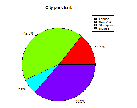
切片百分比和圖表圖例
我們可以透過建立額外的圖表變數來新增切片百分比和圖表圖例。
# Create data for the graph.
x <- c(21, 62, 10,53)
labels <- c("London","New York","Singapore","Mumbai")
piepercent<- round(100*x/sum(x), 1)
# Give the chart file a name.
png(file = "city_percentage_legends.jpg")
# Plot the chart.
pie(x, labels = piepercent, main = "City pie chart",col = rainbow(length(x)))
legend("topright", c("London","New York","Singapore","Mumbai"), cex = 0.8,
fill = rainbow(length(x)))
# Save the file.
dev.off()
當我們執行以上程式碼時,它會產生以下結果:
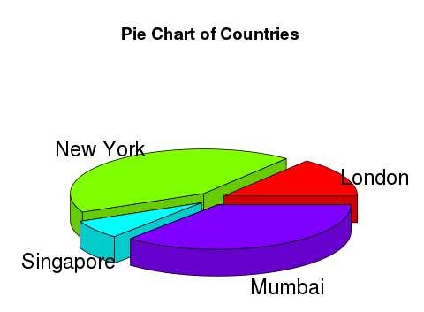
3D 餅圖
可以使用其他包繪製具有 3 個維度的餅圖。plotrix包有一個名為pie3D()的函式用於此。
# Get the library.
library(plotrix)
# Create data for the graph.
x <- c(21, 62, 10,53)
lbl <- c("London","New York","Singapore","Mumbai")
# Give the chart file a name.
png(file = "3d_pie_chart.jpg")
# Plot the chart.
pie3D(x,labels = lbl,explode = 0.1, main = "Pie Chart of Countries ")
# Save the file.
dev.off()
當我們執行以上程式碼時,它會產生以下結果:
R - 條形圖
條形圖以矩形條的形式表示資料,條形的長度與變數的值成正比。R 使用barplot()函式建立條形圖。R 可以在條形圖中繪製垂直和水平條。在條形圖中,每個條都可以賦予不同的顏色。
語法
在 R 中建立條形圖的基本語法為 -
barplot(H,xlab,ylab,main, names.arg,col)
以下是所用引數的描述:
- H是包含條形圖中使用的數值的向量或矩陣。
- xlab是 x 軸的標籤。
- ylab是 y 軸的標籤。
- main是條形圖的標題。
- names.arg是每個條形下方顯示的名稱的向量。
- col用於為圖形中的條形賦予顏色。
示例
一個簡單的條形圖是僅使用輸入向量和每個條形的名稱建立的。
以下指令碼將在當前 R 工作目錄中建立和儲存條形圖。
# Create the data for the chart H <- c(7,12,28,3,41) # Give the chart file a name png(file = "barchart.png") # Plot the bar chart barplot(H) # Save the file dev.off()
當我們執行上述程式碼時,它會產生以下結果 -

條形圖標籤、標題和顏色
可以透過新增更多引數來擴充套件條形圖的特徵。main引數用於新增標題。col引數用於向條形新增顏色。args.name是一個向量,其值數量與輸入向量相同,用於描述每個條形的含義。
示例
以下指令碼將在當前 R 工作目錄中建立和儲存條形圖。
# Create the data for the chart
H <- c(7,12,28,3,41)
M <- c("Mar","Apr","May","Jun","Jul")
# Give the chart file a name
png(file = "barchart_months_revenue.png")
# Plot the bar chart
barplot(H,names.arg=M,xlab="Month",ylab="Revenue",col="blue",
main="Revenue chart",border="red")
# Save the file
dev.off()
當我們執行上述程式碼時,它會產生以下結果 -

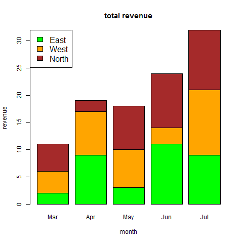
分組條形圖和堆疊條形圖
我們可以透過使用矩陣作為輸入值來建立帶有條形組和每個條形中堆疊的條形圖。
多個變量表示為矩陣,用於建立分組條形圖和堆疊條形圖。
# Create the input vectors.
colors = c("green","orange","brown")
months <- c("Mar","Apr","May","Jun","Jul")
regions <- c("East","West","North")
# Create the matrix of the values.
Values <- matrix(c(2,9,3,11,9,4,8,7,3,12,5,2,8,10,11), nrow = 3, ncol = 5, byrow = TRUE)
# Give the chart file a name
png(file = "barchart_stacked.png")
# Create the bar chart
barplot(Values, main = "total revenue", names.arg = months, xlab = "month", ylab = "revenue", col = colors)
# Add the legend to the chart
legend("topleft", regions, cex = 1.3, fill = colors)
# Save the file
dev.off()
R - 箱線圖
箱線圖是衡量資料集中資料分佈程度的指標。它將資料集分成三個四分位數。此圖形表示資料集中的最小值、最大值、中位數、第一四分位數和第三四分位數。它也有助於透過為每個資料集繪製箱線圖來比較跨資料集的資料分佈。
箱線圖是在 R 中使用boxplot()函式建立的。
語法
在 R 中建立箱線圖的基本語法為 -
boxplot(x, data, notch, varwidth, names, main)
以下是所用引數的描述:
x是向量或公式。
data是資料框。
notch是邏輯值。設定為 TRUE 以繪製凹口。
varwidth是邏輯值。設定為 true 以繪製與樣本量成比例的框寬度。
names是將在每個箱線圖下方列印的組標籤。
main用於為圖形指定標題。
示例
我們使用 R 環境中可用的資料集“mtcars”來建立一個基本的箱線圖。讓我們看一下 mtcars 中的“mpg”和“cyl”列。
input <- mtcars[,c('mpg','cyl')]
print(head(input))
當我們執行上述程式碼時,它會產生以下結果 -
mpg cyl Mazda RX4 21.0 6 Mazda RX4 Wag 21.0 6 Datsun 710 22.8 4 Hornet 4 Drive 21.4 6 Hornet Sportabout 18.7 8 Valiant 18.1 6
建立箱線圖
以下指令碼將為 mpg(每加侖英里數)和 cyl(氣缸數)之間的關係建立一個箱線圖。
# Give the chart file a name. png(file = "boxplot.png") # Plot the chart. boxplot(mpg ~ cyl, data = mtcars, xlab = "Number of Cylinders", ylab = "Miles Per Gallon", main = "Mileage Data") # Save the file. dev.off()
當我們執行以上程式碼時,它會產生以下結果:

帶凹口的箱線圖
我們可以繪製帶凹口的箱線圖,以找出不同資料組的中位數如何相互匹配。
以下指令碼將為每個資料組建立一個帶凹口的箱線圖。
# Give the chart file a name.
png(file = "boxplot_with_notch.png")
# Plot the chart.
boxplot(mpg ~ cyl, data = mtcars,
xlab = "Number of Cylinders",
ylab = "Miles Per Gallon",
main = "Mileage Data",
notch = TRUE,
varwidth = TRUE,
col = c("green","yellow","purple"),
names = c("High","Medium","Low")
)
# Save the file.
dev.off()
當我們執行以上程式碼時,它會產生以下結果:
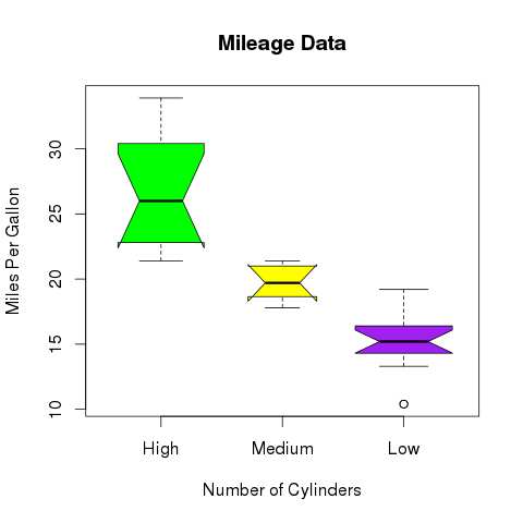
R - 直方圖
直方圖表示變數值的頻率,這些值被分成範圍。直方圖類似於條形圖,但區別在於它將值分組到連續範圍內。直方圖中的每個條形都表示該範圍內存在的數值的高度。
R 使用 **hist()** 函式建立直方圖。此函式以向量作為輸入,並使用一些其他引數來繪製直方圖。
語法
使用 R 建立直方圖的基本語法如下:
hist(v,main,xlab,xlim,ylim,breaks,col,border)
以下是所用引數的描述:
**v** 是一個包含直方圖中使用的數值的向量。
**main** 指示圖表標題。
**col** 用於設定條形的顏色。
**border** 用於設定每個條形的邊框顏色。
**xlab** 用於給出 x 軸的描述。
**xlim** 用於指定 x 軸上的值範圍。
**ylim** 用於指定 y 軸上的值範圍。
**breaks** 用於指定每個條形的寬度。
示例
可以使用輸入向量、標籤、顏色和邊框引數建立一個簡單的直方圖。
下面給出的指令碼將在當前 R 工作目錄中建立並儲存直方圖。
# Create data for the graph. v <- c(9,13,21,8,36,22,12,41,31,33,19) # Give the chart file a name. png(file = "histogram.png") # Create the histogram. hist(v,xlab = "Weight",col = "yellow",border = "blue") # Save the file. dev.off()
當我們執行以上程式碼時,它會產生以下結果:
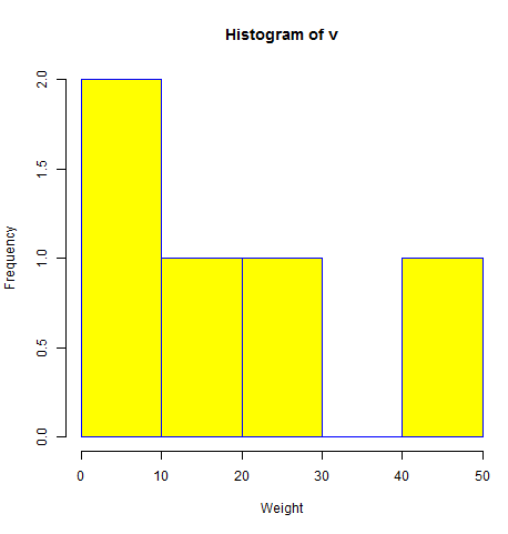
X 和 Y 值的範圍
要指定 X 軸和 Y 軸允許的值範圍,可以使用 xlim 和 ylim 引數。
每個條形的寬度可以透過使用 breaks 來決定。
# Create data for the graph. v <- c(9,13,21,8,36,22,12,41,31,33,19) # Give the chart file a name. png(file = "histogram_lim_breaks.png") # Create the histogram. hist(v,xlab = "Weight",col = "green",border = "red", xlim = c(0,40), ylim = c(0,5), breaks = 5) # Save the file. dev.off()
當我們執行以上程式碼時,它會產生以下結果:
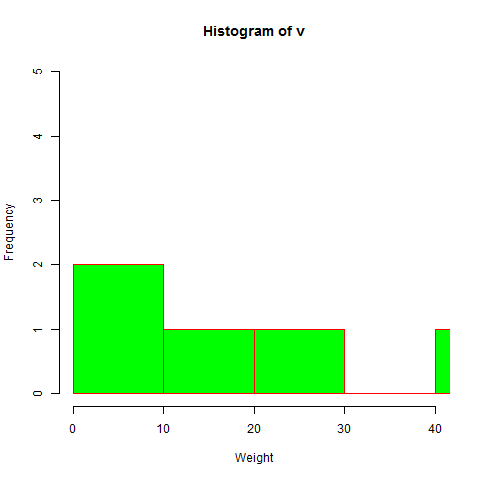
R - 線形圖
折線圖是一種透過在點之間繪製線段來連線一系列點的圖形。這些點按其中一個座標(通常是 x 座標)的值排序。折線圖通常用於識別資料中的趨勢。
R 中的 **plot()** 函式用於建立折線圖。
語法
在 R 中建立折線圖的基本語法如下:
plot(v,type,col,xlab,ylab)
以下是所用引數的描述:
**v** 是一個包含數值的向量。
**type** 取值 "p" 表示僅繪製點,"l" 表示僅繪製線,"o" 表示繪製點和線。
xlab是 x 軸的標籤。
ylab是 y 軸的標籤。
**main** 是圖表的標題。
**col** 用於給點和線著色。
示例
可以使用輸入向量並將 type 引數設定為 "O" 建立一個簡單的折線圖。下面的指令碼將在當前 R 工作目錄中建立並儲存一個折線圖。
# Create the data for the chart. v <- c(7,12,28,3,41) # Give the chart file a name. png(file = "line_chart.jpg") # Plot the bar chart. plot(v,type = "o") # Save the file. dev.off()
當我們執行以上程式碼時,它會產生以下結果:
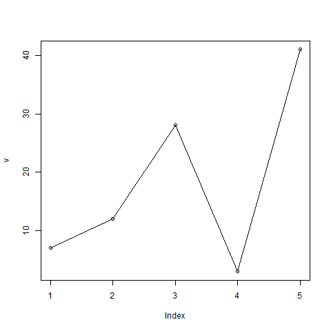
折線圖示題、顏色和標籤
可以透過使用其他引數來擴充套件折線圖的功能。我們可以為點和線新增顏色,為圖表新增標題,併為軸新增標籤。
示例
# Create the data for the chart. v <- c(7,12,28,3,41) # Give the chart file a name. png(file = "line_chart_label_colored.jpg") # Plot the bar chart. plot(v,type = "o", col = "red", xlab = "Month", ylab = "Rain fall", main = "Rain fall chart") # Save the file. dev.off()
當我們執行以上程式碼時,它會產生以下結果:
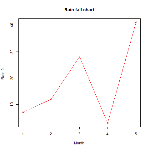
折線圖中的多條線
可以透過使用 **lines()** 函式在同一圖表上繪製多條線。
繪製第一條線後,lines() 函式可以使用一個額外的向量作為輸入來繪製圖表中的第二條線,
# Create the data for the chart. v <- c(7,12,28,3,41) t <- c(14,7,6,19,3) # Give the chart file a name. png(file = "line_chart_2_lines.jpg") # Plot the bar chart. plot(v,type = "o",col = "red", xlab = "Month", ylab = "Rain fall", main = "Rain fall chart") lines(t, type = "o", col = "blue") # Save the file. dev.off()
當我們執行以上程式碼時,它會產生以下結果:
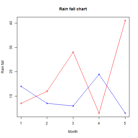
R - 散點圖
散點圖顯示在笛卡爾平面上繪製的許多點。每個點表示兩個變數的值。一個變數選擇在橫軸上,另一個變數選擇在縱軸上。
簡單的散點圖使用 **plot()** 函式建立。
語法
在 R 中建立散點圖的基本語法如下:
plot(x, y, main, xlab, ylab, xlim, ylim, axes)
以下是所用引數的描述:
**x** 是其值為橫座標的資料集。
**y** 是其值為縱座標的資料集。
**main** 是圖形的標題。
**xlab** 是橫軸上的標籤。
**ylab** 是縱軸上的標籤。
**xlim** 是用於繪圖的 x 值的限制。
**ylim** 是用於繪圖的 y 值的限制。
**axes** 指示是否應在繪圖上繪製兩個軸。
示例
我們使用 R 環境中可用的資料集 **"mtcars"** 來建立一個基本的散點圖。讓我們使用 mtcars 中的 "wt" 和 "mpg" 列。
input <- mtcars[,c('wt','mpg')]
print(head(input))
當我們執行以上程式碼時,它會產生以下結果:
wt mpg Mazda RX4 2.620 21.0 Mazda RX4 Wag 2.875 21.0 Datsun 710 2.320 22.8 Hornet 4 Drive 3.215 21.4 Hornet Sportabout 3.440 18.7 Valiant 3.460 18.1
建立散點圖
以下指令碼將為 wt(重量)和 mpg(每加侖英里數)之間的關係建立一個散點圖。
# Get the input values.
input <- mtcars[,c('wt','mpg')]
# Give the chart file a name.
png(file = "scatterplot.png")
# Plot the chart for cars with weight between 2.5 to 5 and mileage between 15 and 30.
plot(x = input$wt,y = input$mpg,
xlab = "Weight",
ylab = "Milage",
xlim = c(2.5,5),
ylim = c(15,30),
main = "Weight vs Milage"
)
# Save the file.
dev.off()
當我們執行以上程式碼時,它會產生以下結果:
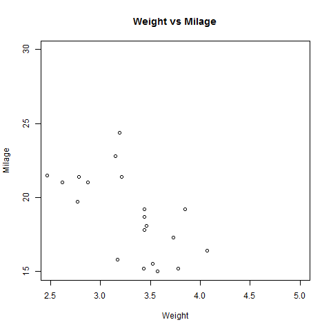
散點圖矩陣
當我們有多個變數並且我們想找到一個變數與其餘變數之間的相關性時,我們使用散點圖矩陣。我們使用 **pairs()** 函式建立散點圖矩陣。
語法
在 R 中建立散點圖矩陣的基本語法如下:
pairs(formula, data)
以下是所用引數的描述:
**formula** 表示成對使用的變數序列。
**data** 表示將從中獲取變數的資料集。
示例
每個變數都與其餘每個變數配對。為每對繪製一個散點圖。
# Give the chart file a name. png(file = "scatterplot_matrices.png") # Plot the matrices between 4 variables giving 12 plots. # One variable with 3 others and total 4 variables. pairs(~wt+mpg+disp+cyl,data = mtcars, main = "Scatterplot Matrix") # Save the file. dev.off()
執行上述程式碼後,我們將得到以下輸出。

R - 均值、中位數和眾數
R 中的統計分析是透過使用許多內建函式來執行的。大多數這些函式都是 R 基礎包的一部分。這些函式將 R 向量作為輸入以及引數,並給出結果。
我們在本章中討論的函式是均值、中位數和眾數。
均值
它是透過將值之和除以資料系列中的值個數來計算的。
**mean()** 函式用於在 R 中計算它。
語法
在 R 中計算均值的基本語法如下:
mean(x, trim = 0, na.rm = FALSE, ...)
以下是所用引數的描述:
**x** 是輸入向量。
**trim** 用於從排序向量的兩端刪除一些觀察值。
**na.rm** 用於從輸入向量中刪除缺失值。
示例
# Create a vector. x <- c(12,7,3,4.2,18,2,54,-21,8,-5) # Find Mean. result.mean <- mean(x) print(result.mean)
當我們執行以上程式碼時,它會產生以下結果:
[1] 8.22
應用 Trim 選項
當提供 trim 引數時,向量中的值將被排序,然後從計算均值中刪除所需數量的觀察值。
當 trim = 0.3 時,將從兩端刪除 3 個值以計算均值。
在這種情況下,排序後的向量為(-21,-5,2,3,4.2,7,8,12,18,54),並且從向量中刪除的值用於計算均值,從左側刪除(-21,-5,2),從右側刪除(12,18,54)。
# Create a vector. x <- c(12,7,3,4.2,18,2,54,-21,8,-5) # Find Mean. result.mean <- mean(x,trim = 0.3) print(result.mean)
當我們執行以上程式碼時,它會產生以下結果:
[1] 5.55
應用 NA 選項
如果存在缺失值,則均值函式將返回 NA。
要從計算中刪除缺失值,請使用 na.rm = TRUE。這意味著刪除 NA 值。
# Create a vector. x <- c(12,7,3,4.2,18,2,54,-21,8,-5,NA) # Find mean. result.mean <- mean(x) print(result.mean) # Find mean dropping NA values. result.mean <- mean(x,na.rm = TRUE) print(result.mean)
當我們執行以上程式碼時,它會產生以下結果:
[1] NA [1] 8.22
中位數
資料系列中最中間的值稱為中位數。**median()** 函式用於在 R 中計算此值。
語法
在 R 中計算中位數的基本語法如下:
median(x, na.rm = FALSE)
以下是所用引數的描述:
**x** 是輸入向量。
**na.rm** 用於從輸入向量中刪除缺失值。
示例
# Create the vector. x <- c(12,7,3,4.2,18,2,54,-21,8,-5) # Find the median. median.result <- median(x) print(median.result)
當我們執行以上程式碼時,它會產生以下結果:
[1] 5.6
眾數
眾數是在一組資料中出現次數最多的值。與均值和中位數不同,眾數可以具有數值資料和字元資料。
R 沒有計算眾數的標準內建函式。因此,我們建立一個使用者函式來計算 R 中資料集的眾數。此函式將向量作為輸入,並將眾數值作為輸出。
示例
# Create the function.
getmode <- function(v) {
uniqv <- unique(v)
uniqv[which.max(tabulate(match(v, uniqv)))]
}
# Create the vector with numbers.
v <- c(2,1,2,3,1,2,3,4,1,5,5,3,2,3)
# Calculate the mode using the user function.
result <- getmode(v)
print(result)
# Create the vector with characters.
charv <- c("o","it","the","it","it")
# Calculate the mode using the user function.
result <- getmode(charv)
print(result)
當我們執行以上程式碼時,它會產生以下結果:
[1] 2 [1] "it"
R - 線性迴歸
迴歸分析是一種非常廣泛使用的統計工具,用於建立兩個變數之間的關係模型。其中一個變數稱為預測變數,其值是透過實驗收集的。另一個變數稱為響應變數,其值是從預測變數匯出的。
線上性迴歸中,這兩個變數透過一個方程相關聯,其中這兩個變數的指數(冪)為 1。從數學上講,線性關係在繪製成圖形時表示一條直線。非線性關係中任何變數的指數都不等於 1,會產生曲線。
線性迴歸的一般數學方程為:
y = ax + b
以下是所用引數的描述:
**y** 是響應變數。
**x** 是預測變數。
**a** 和 **b** 是常數,稱為係數。
建立迴歸的步驟
迴歸的一個簡單示例是預測一個人的體重,已知他的身高。為此,我們需要了解身高和體重之間的關係。
建立關係的步驟如下:
進行實驗以收集身高和相應體重的觀察值的樣本。
使用 R 中的 **lm()** 函式建立關係模型。
從建立的模型中找到係數,並使用這些係數建立數學方程
獲取關係模型的摘要以瞭解預測中的平均誤差。也稱為 **殘差**。
要預測新人的體重,請使用 R 中的 **predict()** 函式。
輸入資料
以下是表示觀察值的樣本資料:
# Values of height 151, 174, 138, 186, 128, 136, 179, 163, 152, 131 # Values of weight. 63, 81, 56, 91, 47, 57, 76, 72, 62, 48
lm() 函式
此函式建立預測變數和響應變數之間的關係模型。
語法
線性迴歸中 **lm()** 函式的基本語法如下:
lm(formula,data)
以下是所用引數的描述:
**formula** 是一個表示 x 和 y 之間關係的符號。
**data** 是將對公式應用的向量。
建立關係模型並獲取係數
x <- c(151, 174, 138, 186, 128, 136, 179, 163, 152, 131) y <- c(63, 81, 56, 91, 47, 57, 76, 72, 62, 48) # Apply the lm() function. relation <- lm(y~x) print(relation)
當我們執行以上程式碼時,它會產生以下結果:
Call: lm(formula = y ~ x) Coefficients: (Intercept) x -38.4551 0.6746
獲取關係的摘要
x <- c(151, 174, 138, 186, 128, 136, 179, 163, 152, 131) y <- c(63, 81, 56, 91, 47, 57, 76, 72, 62, 48) # Apply the lm() function. relation <- lm(y~x) print(summary(relation))
當我們執行以上程式碼時,它會產生以下結果:
Call:
lm(formula = y ~ x)
Residuals:
Min 1Q Median 3Q Max
-6.3002 -1.6629 0.0412 1.8944 3.9775
Coefficients:
Estimate Std. Error t value Pr(>|t|)
(Intercept) -38.45509 8.04901 -4.778 0.00139 **
x 0.67461 0.05191 12.997 1.16e-06 ***
---
Signif. codes: 0 ‘***’ 0.001 ‘**’ 0.01 ‘*’ 0.05 ‘.’ 0.1 ‘ ’ 1
Residual standard error: 3.253 on 8 degrees of freedom
Multiple R-squared: 0.9548, Adjusted R-squared: 0.9491
F-statistic: 168.9 on 1 and 8 DF, p-value: 1.164e-06
predict() 函式
語法
線性迴歸中 predict() 的基本語法如下:
predict(object, newdata)
以下是所用引數的描述:
**object** 是使用 lm() 函式已建立的公式。
**newdata** 是包含預測變數新值的向量。
預測新人的體重
# The predictor vector. x <- c(151, 174, 138, 186, 128, 136, 179, 163, 152, 131) # The resposne vector. y <- c(63, 81, 56, 91, 47, 57, 76, 72, 62, 48) # Apply the lm() function. relation <- lm(y~x) # Find weight of a person with height 170. a <- data.frame(x = 170) result <- predict(relation,a) print(result)
當我們執行以上程式碼時,它會產生以下結果:
1 76.22869
以圖形方式視覺化迴歸
# Create the predictor and response variable. x <- c(151, 174, 138, 186, 128, 136, 179, 163, 152, 131) y <- c(63, 81, 56, 91, 47, 57, 76, 72, 62, 48) relation <- lm(y~x) # Give the chart file a name. png(file = "linearregression.png") # Plot the chart. plot(y,x,col = "blue",main = "Height & Weight Regression", abline(lm(x~y)),cex = 1.3,pch = 16,xlab = "Weight in Kg",ylab = "Height in cm") # Save the file. dev.off()
當我們執行以上程式碼時,它會產生以下結果:
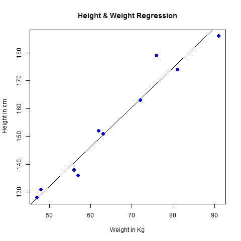
R - 多元迴歸
多元迴歸是線性迴歸擴充套件到兩個以上變數之間關係的擴充套件。在簡單的線性關係中,我們有一個預測變數和一個響應變數,但在多元迴歸中,我們有多個預測變數和一個響應變數。
多元迴歸的一般數學方程為:
y = a + b1x1 + b2x2 +...bnxn
以下是所用引數的描述:
**y** 是響應變數。
**a,b1,b2...bn** 是係數。
**x1,x2,...xn** 是預測變數。
我們使用 R 中的 **lm()** 函式建立迴歸模型。該模型使用輸入資料確定係數的值。接下來,我們可以使用這些係數預測給定一組預測變數時響應變數的值。
lm() 函式
此函式建立預測變數和響應變數之間的關係模型。
語法
多元迴歸中 **lm()** 函式的基本語法如下:
lm(y ~ x1+x2+x3...,data)
以下是所用引數的描述:
**formula** 是一個表示響應變數和預測變數之間關係的符號。
**data** 是將對公式應用的向量。
示例
輸入資料
考慮 R 環境中可用的資料集 "mtcars"。它對不同汽車模型在每加侖英里數(mpg)、汽缸排量("disp")、馬力("hp")、汽車重量("wt")和其他一些引數方面的比較。
模型的目標是建立 "mpg" 作為響應變數與 "disp"、"hp" 和 "wt" 作為預測變數之間的關係。為此,我們建立了這些變數從 mtcars 資料集中提取的子集。
input <- mtcars[,c("mpg","disp","hp","wt")]
print(head(input))
當我們執行以上程式碼時,它會產生以下結果:
mpg disp hp wt Mazda RX4 21.0 160 110 2.620 Mazda RX4 Wag 21.0 160 110 2.875 Datsun 710 22.8 108 93 2.320 Hornet 4 Drive 21.4 258 110 3.215 Hornet Sportabout 18.7 360 175 3.440 Valiant 18.1 225 105 3.460
建立關係模型並獲取係數
input <- mtcars[,c("mpg","disp","hp","wt")]
# Create the relationship model.
model <- lm(mpg~disp+hp+wt, data = input)
# Show the model.
print(model)
# Get the Intercept and coefficients as vector elements.
cat("# # # # The Coefficient Values # # # ","\n")
a <- coef(model)[1]
print(a)
Xdisp <- coef(model)[2]
Xhp <- coef(model)[3]
Xwt <- coef(model)[4]
print(Xdisp)
print(Xhp)
print(Xwt)
當我們執行以上程式碼時,它會產生以下結果:
Call:
lm(formula = mpg ~ disp + hp + wt, data = input)
Coefficients:
(Intercept) disp hp wt
37.105505 -0.000937 -0.031157 -3.800891
# # # # The Coefficient Values # # #
(Intercept)
37.10551
disp
-0.0009370091
hp
-0.03115655
wt
-3.800891
建立迴歸模型方程
根據上述截距和係數值,我們建立數學方程。
Y = a+Xdisp.x1+Xhp.x2+Xwt.x3 or Y = 37.15+(-0.000937)*x1+(-0.0311)*x2+(-3.8008)*x3
應用方程預測新值
我們可以使用上面建立的迴歸方程來預測當提供排量、馬力和重量的新值集時的里程數。
對於一輛 disp = 221、hp = 102 和 wt = 2.91 的汽車,預測的里程數為:
Y = 37.15+(-0.000937)*221+(-0.0311)*102+(-3.8008)*2.91 = 22.7104
R - Logistic 迴歸
邏輯迴歸是一種迴歸模型,其中響應變數(因變數)具有分類值,例如真/假或 0/1。它實際上是根據將響應變數與其預測變數相關聯的數學方程,測量二元響應的機率作為響應變數的值。
邏輯迴歸的一般數學方程為:
y = 1/(1+e^-(a+b1x1+b2x2+b3x3+...))
以下是所用引數的描述:
**y** 是響應變數。
**x** 是預測變數。
**a** 和 **b** 是數值常數係數。
用於建立迴歸模型的函式是glm()函式。
語法
邏輯迴歸中glm()函式的基本語法如下:
glm(formula,data,family)
以下是所用引數的描述:
formula是表示變數之間關係的符號。
data是提供這些變數值的資料集。
family是R物件,用於指定模型的詳細資訊。對於邏輯迴歸,其值為binomial。
示例
內建資料集“mtcars”描述了不同型號汽車及其各種發動機規格。在“mtcars”資料集中,傳輸模式(自動或手動)由列am描述,它是一個二進位制值(0或1)。我們可以建立“am”列與其他3列(hp、wt和cyl)之間的邏輯迴歸模型。
# Select some columns form mtcars.
input <- mtcars[,c("am","cyl","hp","wt")]
print(head(input))
當我們執行以上程式碼時,它會產生以下結果:
am cyl hp wt Mazda RX4 1 6 110 2.620 Mazda RX4 Wag 1 6 110 2.875 Datsun 710 1 4 93 2.320 Hornet 4 Drive 0 6 110 3.215 Hornet Sportabout 0 8 175 3.440 Valiant 0 6 105 3.460
建立迴歸模型
我們使用glm()函式建立迴歸模型並獲取其摘要以進行分析。
input <- mtcars[,c("am","cyl","hp","wt")]
am.data = glm(formula = am ~ cyl + hp + wt, data = input, family = binomial)
print(summary(am.data))
當我們執行以上程式碼時,它會產生以下結果:
Call:
glm(formula = am ~ cyl + hp + wt, family = binomial, data = input)
Deviance Residuals:
Min 1Q Median 3Q Max
-2.17272 -0.14907 -0.01464 0.14116 1.27641
Coefficients:
Estimate Std. Error z value Pr(>|z|)
(Intercept) 19.70288 8.11637 2.428 0.0152 *
cyl 0.48760 1.07162 0.455 0.6491
hp 0.03259 0.01886 1.728 0.0840 .
wt -9.14947 4.15332 -2.203 0.0276 *
---
Signif. codes: 0 ‘***’ 0.001 ‘**’ 0.01 ‘*’ 0.05 ‘.’ 0.1 ‘ ’ 1
(Dispersion parameter for binomial family taken to be 1)
Null deviance: 43.2297 on 31 degrees of freedom
Residual deviance: 9.8415 on 28 degrees of freedom
AIC: 17.841
Number of Fisher Scoring iterations: 8
結論
在摘要中,由於最後一列中變數“cyl”和“hp”的p值大於0.05,因此我們認為它們對變數“am”的值貢獻不顯著。只有重量(wt)會影響此迴歸模型中的“am”值。
R - 正態分佈
在從獨立來源隨機收集的資料中,通常觀察到資料的分佈是正態的。這意味著,在以變數值為橫軸,值的計數為縱軸繪製圖形時,我們會得到一條鐘形曲線。曲線的中心代表資料集的平均值。在圖中,50%的值位於平均值的左側,另外50%的值位於圖形的右側。這在統計學中被稱為正態分佈。
R有四個內建函式來生成正態分佈。它們描述如下。
dnorm(x, mean, sd) pnorm(x, mean, sd) qnorm(p, mean, sd) rnorm(n, mean, sd)
以下是上述函式中使用的引數的描述:
x是數字向量。
p是機率向量。
n是觀測值的數量(樣本量)。
mean是樣本資料的平均值。其預設值為零。
sd是標準差。其預設值為1。
dnorm()
此函式給定均值和標準差,給出每個點處機率分佈的高度。
# Create a sequence of numbers between -10 and 10 incrementing by 0.1. x <- seq(-10, 10, by = .1) # Choose the mean as 2.5 and standard deviation as 0.5. y <- dnorm(x, mean = 2.5, sd = 0.5) # Give the chart file a name. png(file = "dnorm.png") plot(x,y) # Save the file. dev.off()
當我們執行以上程式碼時,它會產生以下結果:
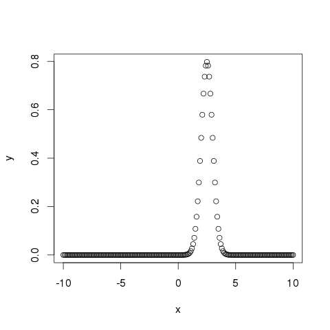
pnorm()
此函式給出正態分佈隨機數小於給定數字的值的機率。它也稱為“累積分佈函式”。
# Create a sequence of numbers between -10 and 10 incrementing by 0.2. x <- seq(-10,10,by = .2) # Choose the mean as 2.5 and standard deviation as 2. y <- pnorm(x, mean = 2.5, sd = 2) # Give the chart file a name. png(file = "pnorm.png") # Plot the graph. plot(x,y) # Save the file. dev.off()
當我們執行以上程式碼時,它會產生以下結果:
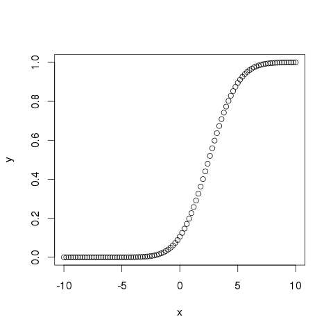
qnorm()
此函式獲取機率值並給出一個累積值與機率值匹配的數字。
# Create a sequence of probability values incrementing by 0.02. x <- seq(0, 1, by = 0.02) # Choose the mean as 2 and standard deviation as 3. y <- qnorm(x, mean = 2, sd = 1) # Give the chart file a name. png(file = "qnorm.png") # Plot the graph. plot(x,y) # Save the file. dev.off()
當我們執行以上程式碼時,它會產生以下結果:

rnorm()
此函式用於生成分佈為正態的隨機數。它以樣本量作為輸入並生成這麼多隨機數。我們繪製直方圖以顯示生成數字的分佈。
# Create a sample of 50 numbers which are normally distributed. y <- rnorm(50) # Give the chart file a name. png(file = "rnorm.png") # Plot the histogram for this sample. hist(y, main = "Normal DIstribution") # Save the file. dev.off()
當我們執行以上程式碼時,它會產生以下結果:
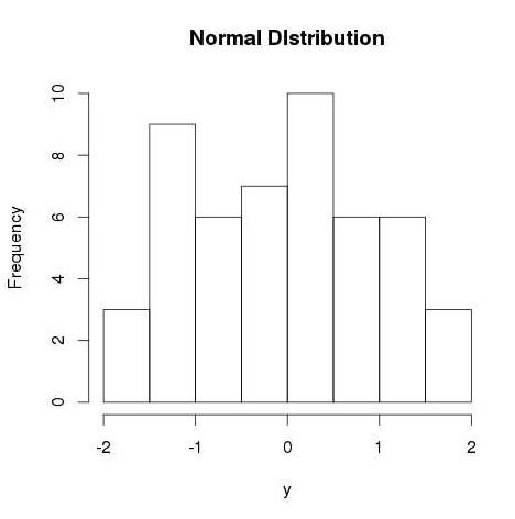
R - 二項分佈
二項分佈模型處理的是在一個系列實驗中,找到一個只有兩個可能結果的事件成功的機率。例如,拋硬幣總是得到正面或反面。在連續拋硬幣10次的情況下,找到正好3個正面的機率是在二項分佈期間估計的。
R有四個內建函式來生成二項分佈。它們描述如下。
dbinom(x, size, prob) pbinom(x, size, prob) qbinom(p, size, prob) rbinom(n, size, prob)
以下是所用引數的描述:
x是數字向量。
p是機率向量。
n是觀測值的數量。
size是試驗次數。
prob是每次試驗成功的機率。
dbinom()
此函式給出每個點處的機率密度分佈。
# Create a sample of 50 numbers which are incremented by 1. x <- seq(0,50,by = 1) # Create the binomial distribution. y <- dbinom(x,50,0.5) # Give the chart file a name. png(file = "dbinom.png") # Plot the graph for this sample. plot(x,y) # Save the file. dev.off()
當我們執行以上程式碼時,它會產生以下結果:
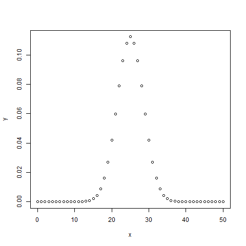
pbinom()
此函式給出事件的累積機率。它是一個表示機率的單個值。
# Probability of getting 26 or less heads from a 51 tosses of a coin. x <- pbinom(26,51,0.5) print(x)
當我們執行以上程式碼時,它會產生以下結果:
[1] 0.610116
qbinom()
此函式獲取機率值並給出一個累積值與機率值匹配的數字。
# How many heads will have a probability of 0.25 will come out when a coin # is tossed 51 times. x <- qbinom(0.25,51,1/2) print(x)
當我們執行以上程式碼時,它會產生以下結果:
[1] 23
rbinom()
此函式從給定樣本中生成給定機率的所需數量的隨機值。
# Find 8 random values from a sample of 150 with probability of 0.4. x <- rbinom(8,150,.4) print(x)
當我們執行以上程式碼時,它會產生以下結果:
[1] 58 61 59 66 55 60 61 67
R - 泊松迴歸
泊松迴歸涉及響應變數以計數形式而不是分數形式表示的迴歸模型。例如,出生人數或足球比賽系列中獲勝次數的計數。此外,響應變數的值遵循泊松分佈。
泊松迴歸的一般數學方程為:
log(y) = a + b1x1 + b2x2 + bnxn.....
以下是所用引數的描述:
**y** 是響應變數。
a和b是數值係數。
**x** 是預測變數。
用於建立泊松迴歸模型的函式是glm()函式。
語法
泊松迴歸中glm()函式的基本語法如下:
glm(formula,data,family)
以下是上述函式中使用的引數的描述:
formula是表示變數之間關係的符號。
data是提供這些變數值的資料集。
family是R物件,用於指定模型的詳細資訊。對於邏輯迴歸,其值為“Poisson”。
示例
我們有內建資料集“warpbreaks”,它描述了羊毛型別(A或B)和張力(低、中或高)對每臺織布機斷紗次數的影響。讓我們將“breaks”視為響應變數,它是斷紗次數的計數。羊毛“type”和“tension”被視為預測變數。
輸入資料
input <- warpbreaks print(head(input))
當我們執行以上程式碼時,它會產生以下結果:
breaks wool tension 1 26 A L 2 30 A L 3 54 A L 4 25 A L 5 70 A L 6 52 A L
建立迴歸模型
output <-glm(formula = breaks ~ wool+tension, data = warpbreaks, family = poisson) print(summary(output))
當我們執行以上程式碼時,它會產生以下結果:
Call:
glm(formula = breaks ~ wool + tension, family = poisson, data = warpbreaks)
Deviance Residuals:
Min 1Q Median 3Q Max
-3.6871 -1.6503 -0.4269 1.1902 4.2616
Coefficients:
Estimate Std. Error z value Pr(>|z|)
(Intercept) 3.69196 0.04541 81.302 < 2e-16 ***
woolB -0.20599 0.05157 -3.994 6.49e-05 ***
tensionM -0.32132 0.06027 -5.332 9.73e-08 ***
tensionH -0.51849 0.06396 -8.107 5.21e-16 ***
---
Signif. codes: 0 ‘***’ 0.001 ‘**’ 0.01 ‘*’ 0.05 ‘.’ 0.1 ‘ ’ 1
(Dispersion parameter for poisson family taken to be 1)
Null deviance: 297.37 on 53 degrees of freedom
Residual deviance: 210.39 on 50 degrees of freedom
AIC: 493.06
Number of Fisher Scoring iterations: 4
在摘要中,我們尋找最後一列中的p值是否小於0.05,以考慮預測變數對響應變數的影響。如所見,張力型別為M和H的羊毛型別B會影響斷紗次數。
R - 協方差分析
我們使用迴歸分析來建立模型,這些模型描述了預測變數變化對響應變數的影響。有時,如果我們有一個分類變數,其值如是/否或男/女等。簡單的迴歸分析會為分類變數的每個值提供多個結果。在這種情況下,我們可以透過將分類變數與預測變數一起使用並比較分類變數每個水平的迴歸線來研究分類變數的影響。這種分析被稱為協方差分析,也稱為ANCOVA。
示例
考慮R內建資料集mtcars。在其中,我們觀察到欄位“am”表示傳輸型別(自動或手動)。它是一個分類變數,其值為0和1。汽車的每加侖英里數(mpg)除了馬力("hp")的值外,也可能取決於它。
我們研究“am”的值對“mpg”和“hp”之間迴歸的影響。這是透過使用aov()函式,然後使用anova()函式來比較多個迴歸來完成的。
輸入資料
建立一個包含資料集mtcars中的“mpg”、“hp”和“am”欄位的資料框。在這裡,我們將“mpg”作為響應變數,“hp”作為預測變數,“am”作為分類變數。
input <- mtcars[,c("am","mpg","hp")]
print(head(input))
當我們執行以上程式碼時,它會產生以下結果:
am mpg hp Mazda RX4 1 21.0 110 Mazda RX4 Wag 1 21.0 110 Datsun 710 1 22.8 93 Hornet 4 Drive 0 21.4 110 Hornet Sportabout 0 18.7 175 Valiant 0 18.1 105
ANCOVA分析
我們建立一個迴歸模型,將“hp”作為預測變數,將“mpg”作為響應變數,並考慮“am”和“hp”之間的互動作用。
具有分類變數和預測變數之間互動作用的模型
# Get the dataset. input <- mtcars # Create the regression model. result <- aov(mpg~hp*am,data = input) print(summary(result))
當我們執行以上程式碼時,它會產生以下結果:
Df Sum Sq Mean Sq F value Pr(>F) hp 1 678.4 678.4 77.391 1.50e-09 *** am 1 202.2 202.2 23.072 4.75e-05 *** hp:am 1 0.0 0.0 0.001 0.981 Residuals 28 245.4 8.8 --- Signif. codes: 0 ‘***’ 0.001 ‘**’ 0.01 ‘*’ 0.05 ‘.’ 0.1 ‘ ’ 1
此結果表明,馬力和傳輸型別都對每加侖英里數有顯著影響,因為在這兩種情況下,p值都小於0.05。但是,這兩個變數之間的互動作用並不顯著,因為p值大於0.05。
沒有分類變數和預測變數之間互動作用的模型
# Get the dataset. input <- mtcars # Create the regression model. result <- aov(mpg~hp+am,data = input) print(summary(result))
當我們執行以上程式碼時,它會產生以下結果:
Df Sum Sq Mean Sq F value Pr(>F) hp 1 678.4 678.4 80.15 7.63e-10 *** am 1 202.2 202.2 23.89 3.46e-05 *** Residuals 29 245.4 8.5 --- Signif. codes: 0 ‘***’ 0.001 ‘**’ 0.01 ‘*’ 0.05 ‘.’ 0.1 ‘ ’ 1
此結果表明,馬力和傳輸型別都對每加侖英里數有顯著影響,因為在這兩種情況下,p值都小於0.05。
比較兩個模型
現在我們可以比較這兩個模型,以得出變數的互動作用是否確實不顯著的結論。為此,我們使用anova()函式。
# Get the dataset. input <- mtcars # Create the regression models. result1 <- aov(mpg~hp*am,data = input) result2 <- aov(mpg~hp+am,data = input) # Compare the two models. print(anova(result1,result2))
當我們執行以上程式碼時,它會產生以下結果:
Model 1: mpg ~ hp * am Model 2: mpg ~ hp + am Res.Df RSS Df Sum of Sq F Pr(>F) 1 28 245.43 2 29 245.44 -1 -0.0052515 6e-04 0.9806
由於p值大於0.05,因此我們得出結論,馬力和傳輸型別之間的互動作用不顯著。因此,在自動和手動傳輸模式下,每加侖英里數將以類似的方式取決於汽車的馬力。
R - 時間序列分析
時間序列是一系列資料點,其中每個資料點都與一個時間戳相關聯。一個簡單的例子是股票市場中某隻股票在給定日期的不同時間點的價格。另一個例子是某一地區不同月份的降雨量。R語言使用許多函式來建立、操作和繪製時間序列資料。時間序列的資料儲存在一個稱為時間序列物件的R物件中。它也是一個R資料物件,如向量或資料框。
時間序列物件是透過使用ts()函式建立的。
語法
時間序列分析中ts()函式的基本語法如下:
timeseries.object.name <- ts(data, start, end, frequency)
以下是所用引數的描述:
data是包含時間序列中使用的值的向量或矩陣。
start指定時間序列中第一個觀測值的開始時間。
end指定時間序列中最後一個觀測值的結束時間。
frequency指定每個單位時間的觀測值數量。
除了引數“data”之外,所有其他引數都是可選的。
示例
考慮從2012年1月開始某地的年降雨量詳細資訊。我們為期12個月建立一個R時間序列物件並繪製它。
# Get the data points in form of a R vector. rainfall <- c(799,1174.8,865.1,1334.6,635.4,918.5,685.5,998.6,784.2,985,882.8,1071) # Convert it to a time series object. rainfall.timeseries <- ts(rainfall,start = c(2012,1),frequency = 12) # Print the timeseries data. print(rainfall.timeseries) # Give the chart file a name. png(file = "rainfall.png") # Plot a graph of the time series. plot(rainfall.timeseries) # Save the file. dev.off()
當我們執行上述程式碼時,它會產生以下結果和圖表:
Jan Feb Mar Apr May Jun Jul Aug Sep
2012 799.0 1174.8 865.1 1334.6 635.4 918.5 685.5 998.6 784.2
Oct Nov Dec
2012 985.0 882.8 1071.0
時間序列圖表:
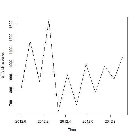
不同的時間間隔
ts()函式中frequency引數的值決定了測量資料點的時段。值為12表示時間序列為12個月。其他值及其含義如下:
frequency = 12將資料點固定在每年的每個月。
frequency = 4將資料點固定在每年的每個季度。
frequency = 6將資料點固定在每小時的每10分鐘。
frequency = 24*6將資料點固定在每天的每10分鐘。
多個時間序列
我們可以透過將兩個序列組合成一個矩陣,在一個圖表中繪製多個時間序列。
# Get the data points in form of a R vector.
rainfall1 <- c(799,1174.8,865.1,1334.6,635.4,918.5,685.5,998.6,784.2,985,882.8,1071)
rainfall2 <-
c(655,1306.9,1323.4,1172.2,562.2,824,822.4,1265.5,799.6,1105.6,1106.7,1337.8)
# Convert them to a matrix.
combined.rainfall <- matrix(c(rainfall1,rainfall2),nrow = 12)
# Convert it to a time series object.
rainfall.timeseries <- ts(combined.rainfall,start = c(2012,1),frequency = 12)
# Print the timeseries data.
print(rainfall.timeseries)
# Give the chart file a name.
png(file = "rainfall_combined.png")
# Plot a graph of the time series.
plot(rainfall.timeseries, main = "Multiple Time Series")
# Save the file.
dev.off()
當我們執行上述程式碼時,它會產生以下結果和圖表:
Series 1 Series 2 Jan 2012 799.0 655.0 Feb 2012 1174.8 1306.9 Mar 2012 865.1 1323.4 Apr 2012 1334.6 1172.2 May 2012 635.4 562.2 Jun 2012 918.5 824.0 Jul 2012 685.5 822.4 Aug 2012 998.6 1265.5 Sep 2012 784.2 799.6 Oct 2012 985.0 1105.6 Nov 2012 882.8 1106.7 Dec 2012 1071.0 1337.8
多個時間序列圖表:
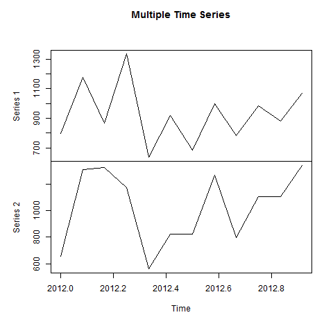
R - 非線性最小二乘法
在對迴歸分析的現實世界資料進行建模時,我們觀察到模型的方程很少是線性方程,給出線性圖。大多數情況下,現實世界資料的模型方程涉及更高次方的數學函式,如3的指數或正弦函式。在這種情況下,模型的圖給出的是曲線而不是直線。線性迴歸和非線性迴歸的目標都是調整模型引數的值,以找到最接近資料的直線或曲線。找到這些值後,我們將能夠以良好的精度估計響應變數。
在最小二乘迴歸中,我們建立一個迴歸模型,其中不同點到迴歸曲線的垂直距離的平方和最小化。我們通常從一個定義的模型開始,併為係數假設一些值。然後,我們應用R的nls()函式來獲得更準確的值以及置信區間。
語法
在R中建立非線性最小二乘檢驗的基本語法如下:
nls(formula, data, start)
以下是所用引數的描述:
formula是非線性模型公式,包括變數和引數。
data是用於評估公式中變數的資料框。
start是起始估計的命名列表或命名數值向量。
示例
我們將考慮一個非線性模型,並假設其係數的初始值。接下來,我們將瞭解這些假設值的置信區間是什麼,以便我們可以判斷這些值與模型的擬合程度。
因此,讓我們考慮以下方程以達到此目的:
a = b1*x^2+b2
讓我們假設初始係數為1和3,並將這些值擬合到nls()函式中。
xvalues <- c(1.6,2.1,2,2.23,3.71,3.25,3.4,3.86,1.19,2.21) yvalues <- c(5.19,7.43,6.94,8.11,18.75,14.88,16.06,19.12,3.21,7.58) # Give the chart file a name. png(file = "nls.png") # Plot these values. plot(xvalues,yvalues) # Take the assumed values and fit into the model. model <- nls(yvalues ~ b1*xvalues^2+b2,start = list(b1 = 1,b2 = 3)) # Plot the chart with new data by fitting it to a prediction from 100 data points. new.data <- data.frame(xvalues = seq(min(xvalues),max(xvalues),len = 100)) lines(new.data$xvalues,predict(model,newdata = new.data)) # Save the file. dev.off() # Get the sum of the squared residuals. print(sum(resid(model)^2)) # Get the confidence intervals on the chosen values of the coefficients. print(confint(model))
當我們執行以上程式碼時,它會產生以下結果:
[1] 1.081935
Waiting for profiling to be done...
2.5% 97.5%
b1 1.137708 1.253135
b2 1.497364 2.496484
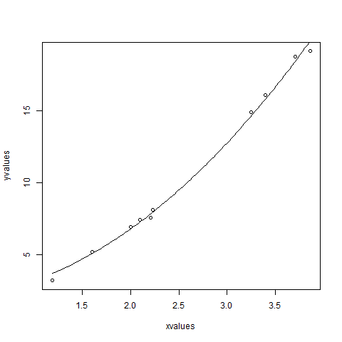
我們可以得出結論,b1的值更接近1,而b2的值更接近2而不是3。
R - 決策樹
決策樹是一個圖形,用於以樹的形式表示選擇及其結果。圖中的節點表示事件或選擇,圖的邊表示決策規則或條件。它主要用於使用R的機器學習和資料探勘應用程式。
決策樹的應用示例包括:預測電子郵件是否為垃圾郵件,預測腫瘤是否為癌性,或根據貸款的相關因素預測貸款信用風險的好壞。通常,模型是使用觀察到的資料(也稱為訓練資料)建立的。然後,使用一組驗證資料來驗證和改進模型。R 擁有用於建立和視覺化決策樹的包。對於新的預測變數集,我們使用此模型來確定資料的類別(是/否,垃圾郵件/非垃圾郵件)。
R 包 "party" 用於建立決策樹。
安裝 R 包
在 R 控制檯中使用以下命令安裝該包。如有任何依賴包,您也需要安裝它們。
install.packages("party")
包 "party" 包含函式 ctree(),用於建立和分析決策樹。
語法
在 R 中建立決策樹的基本語法如下:
ctree(formula, data)
以下是所用引數的描述:
formula 是一個描述預測變數和響應變數的公式。
data 是所用資料集的名稱。
輸入資料
我們將使用名為 readingSkills 的 R 內建資料集來建立決策樹。如果我們知道變數“age”(年齡),“shoesize”(鞋碼),“score”(分數)以及該人是否為母語人士,它描述了某人閱讀技能分數。
以下是樣本資料。
# Load the party package. It will automatically load other # dependent packages. library(party) # Print some records from data set readingSkills. print(head(readingSkills))
當我們執行上述程式碼時,它會產生以下結果和圖表:
nativeSpeaker age shoeSize score 1 yes 5 24.83189 32.29385 2 yes 6 25.95238 36.63105 3 no 11 30.42170 49.60593 4 yes 7 28.66450 40.28456 5 yes 11 31.88207 55.46085 6 yes 10 30.07843 52.83124 Loading required package: methods Loading required package: grid ............................... ...............................
示例
我們將使用 ctree() 函式建立決策樹並檢視其圖形。
# Load the party package. It will automatically load other # dependent packages. library(party) # Create the input data frame. input.dat <- readingSkills[c(1:105),] # Give the chart file a name. png(file = "decision_tree.png") # Create the tree. output.tree <- ctree( nativeSpeaker ~ age + shoeSize + score, data = input.dat) # Plot the tree. plot(output.tree) # Save the file. dev.off()
當我們執行以上程式碼時,它會產生以下結果:
null device
1
Loading required package: methods
Loading required package: grid
Loading required package: mvtnorm
Loading required package: modeltools
Loading required package: stats4
Loading required package: strucchange
Loading required package: zoo
Attaching package: ‘zoo’
The following objects are masked from ‘package:base’:
as.Date, as.Date.numeric
Loading required package: sandwich
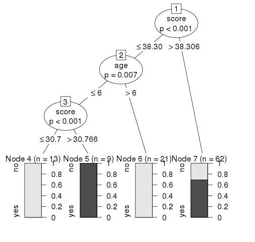
結論
從上面顯示的決策樹中,我們可以得出結論,任何閱讀技能分數小於 38.3 且年齡大於 6 的人都不是母語人士。
R - 隨機森林
在隨機森林方法中,會建立大量的決策樹。每個觀察值都會輸入到每個決策樹中。每個觀察值最常見的輸出用作最終輸出。將新的觀察值輸入到所有樹中,並對每個分類模型進行多數投票。
對構建樹時未使用的案例進行誤差估計。這稱為 OOB(袋外) 誤差估計,以百分比表示。
R 包 "randomForest" 用於建立隨機森林。
安裝 R 包
在 R 控制檯中使用以下命令安裝該包。如有任何依賴包,您也需要安裝它們。
install.packages("randomForest)
包 "randomForest" 包含函式 randomForest(),用於建立和分析隨機森林。
語法
在 R 中建立隨機森林的基本語法如下:
randomForest(formula, data)
以下是所用引數的描述:
formula 是一個描述預測變數和響應變數的公式。
data 是所用資料集的名稱。
輸入資料
我們將使用名為 readingSkills 的 R 內建資料集來建立決策樹。它描述了某人閱讀技能的分數,如果我們知道變數“age”(年齡),“shoesize”(鞋碼),“score”(分數)以及該人是否為母語人士。
以下是樣本資料。
# Load the party package. It will automatically load other # required packages. library(party) # Print some records from data set readingSkills. print(head(readingSkills))
當我們執行上述程式碼時,它會產生以下結果和圖表:
nativeSpeaker age shoeSize score 1 yes 5 24.83189 32.29385 2 yes 6 25.95238 36.63105 3 no 11 30.42170 49.60593 4 yes 7 28.66450 40.28456 5 yes 11 31.88207 55.46085 6 yes 10 30.07843 52.83124 Loading required package: methods Loading required package: grid ............................... ...............................
示例
我們將使用 randomForest() 函式建立決策樹並檢視其圖形。
# Load the party package. It will automatically load other
# required packages.
library(party)
library(randomForest)
# Create the forest.
output.forest <- randomForest(nativeSpeaker ~ age + shoeSize + score,
data = readingSkills)
# View the forest results.
print(output.forest)
# Importance of each predictor.
print(importance(fit,type = 2))
當我們執行以上程式碼時,它會產生以下結果:
Call:
randomForest(formula = nativeSpeaker ~ age + shoeSize + score,
data = readingSkills)
Type of random forest: classification
Number of trees: 500
No. of variables tried at each split: 1
OOB estimate of error rate: 1%
Confusion matrix:
no yes class.error
no 99 1 0.01
yes 1 99 0.01
MeanDecreaseGini
age 13.95406
shoeSize 18.91006
score 56.73051
結論
從上面顯示的隨機森林中,我們可以得出結論,鞋碼和分數是決定某人是否為母語人士的重要因素。此外,模型只有 1% 的誤差,這意味著我們可以以 99% 的準確率進行預測。
R - 生存分析
生存分析涉及預測特定事件將發生的時間。它也稱為失效時間分析或死亡時間分析。例如,預測癌症患者的生存天數或預測機械系統何時會發生故障。
名為 survival 的 R 包用於執行生存分析。此包包含函式 Surv(),它將輸入資料作為 R 公式,並在選定的變數之間建立一個生存物件以進行分析。然後,我們使用函式 survfit() 為分析建立圖表。
安裝包
install.packages("survival")
語法
在 R 中建立生存分析的基本語法如下:
Surv(time,event) survfit(formula)
以下是所用引數的描述:
time 是事件發生前的隨訪時間。
event 指示預期事件發生的狀態。
formula 是預測變數之間的關係。
示例
我們將考慮名為“pbc”的資料集,該資料集存在於上面安裝的 survival 包中。它描述了患有原發性膽汁性肝硬化 (PBC) 的患者的生存資料點。在資料集中存在的許多列中,我們主要關注“time”和“status”欄位。Time 表示患者註冊和患者接受肝移植或患者死亡之間較早事件之間的時間(以天為單位)。
# Load the library.
library("survival")
# Print first few rows.
print(head(pbc))
當我們執行上述程式碼時,它會產生以下結果和圖表:
id time status trt age sex ascites hepato spiders edema bili chol 1 1 400 2 1 58.76523 f 1 1 1 1.0 14.5 261 2 2 4500 0 1 56.44627 f 0 1 1 0.0 1.1 302 3 3 1012 2 1 70.07255 m 0 0 0 0.5 1.4 176 4 4 1925 2 1 54.74059 f 0 1 1 0.5 1.8 244 5 5 1504 1 2 38.10541 f 0 1 1 0.0 3.4 279 6 6 2503 2 2 66.25873 f 0 1 0 0.0 0.8 248 albumin copper alk.phos ast trig platelet protime stage 1 2.60 156 1718.0 137.95 172 190 12.2 4 2 4.14 54 7394.8 113.52 88 221 10.6 3 3 3.48 210 516.0 96.10 55 151 12.0 4 4 2.54 64 6121.8 60.63 92 183 10.3 4 5 3.53 143 671.0 113.15 72 136 10.9 3 6 3.98 50 944.0 93.00 63 NA 11.0 3
從上述資料中,我們正在考慮時間和狀態進行分析。
應用 Surv() 和 survfit() 函式
現在我們繼續將 Surv() 函式應用於上述資料集,並建立一個圖表以顯示趨勢。
# Load the library.
library("survival")
# Create the survival object.
survfit(Surv(pbc$time,pbc$status == 2)~1)
# Give the chart file a name.
png(file = "survival.png")
# Plot the graph.
plot(survfit(Surv(pbc$time,pbc$status == 2)~1))
# Save the file.
dev.off()
當我們執行上述程式碼時,它會產生以下結果和圖表:
Call: survfit(formula = Surv(pbc$time, pbc$status == 2) ~ 1)
n events median 0.95LCL 0.95UCL
418 161 3395 3090 3853
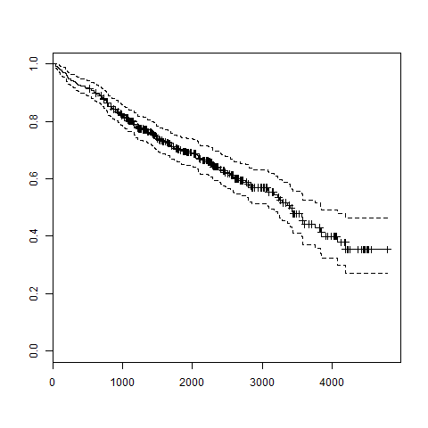
上圖中的趨勢有助於我們預測在一定天數結束時生存的機率。
R - 卡方檢驗
卡方檢驗是一種統計方法,用於確定兩個分類變數之間是否存在顯著的相關性。這兩個變數都應來自同一總體,並且應為分類變數,例如:是/否,男/女,紅/綠等。
例如,我們可以構建一個包含人們冰淇淋購買模式觀察值的資料集,並嘗試將一個人的性別與其偏好的冰淇淋口味相關聯。如果發現相關性,我們可以通過了解訪客的性別數量來計劃相應口味的庫存。
語法
執行卡方檢驗的函式為 chisq.test()。
在 R 中建立卡方檢驗的基本語法如下:
chisq.test(data)
以下是所用引數的描述:
data 是表格形式的資料,包含觀察中變數的計數值。
示例
我們將使用 "MASS" 庫中的 Cars93 資料,它表示 1993 年不同汽車型號的銷量。
library("MASS")
print(str(Cars93))
當我們執行以上程式碼時,它會產生以下結果:
'data.frame': 93 obs. of 27 variables: $ Manufacturer : Factor w/ 32 levels "Acura","Audi",..: 1 1 2 2 3 4 4 4 4 5 ... $ Model : Factor w/ 93 levels "100","190E","240",..: 49 56 9 1 6 24 54 74 73 35 ... $ Type : Factor w/ 6 levels "Compact","Large",..: 4 3 1 3 3 3 2 2 3 2 ... $ Min.Price : num 12.9 29.2 25.9 30.8 23.7 14.2 19.9 22.6 26.3 33 ... $ Price : num 15.9 33.9 29.1 37.7 30 15.7 20.8 23.7 26.3 34.7 ... $ Max.Price : num 18.8 38.7 32.3 44.6 36.2 17.3 21.7 24.9 26.3 36.3 ... $ MPG.city : int 25 18 20 19 22 22 19 16 19 16 ... $ MPG.highway : int 31 25 26 26 30 31 28 25 27 25 ... $ AirBags : Factor w/ 3 levels "Driver & Passenger",..: 3 1 2 1 2 2 2 2 2 2 ... $ DriveTrain : Factor w/ 3 levels "4WD","Front",..: 2 2 2 2 3 2 2 3 2 2 ... $ Cylinders : Factor w/ 6 levels "3","4","5","6",..: 2 4 4 4 2 2 4 4 4 5 ... $ EngineSize : num 1.8 3.2 2.8 2.8 3.5 2.2 3.8 5.7 3.8 4.9 ... $ Horsepower : int 140 200 172 172 208 110 170 180 170 200 ... $ RPM : int 6300 5500 5500 5500 5700 5200 4800 4000 4800 4100 ... $ Rev.per.mile : int 2890 2335 2280 2535 2545 2565 1570 1320 1690 1510 ... $ Man.trans.avail : Factor w/ 2 levels "No","Yes": 2 2 2 2 2 1 1 1 1 1 ... $ Fuel.tank.capacity: num 13.2 18 16.9 21.1 21.1 16.4 18 23 18.8 18 ... $ Passengers : int 5 5 5 6 4 6 6 6 5 6 ... $ Length : int 177 195 180 193 186 189 200 216 198 206 ... $ Wheelbase : int 102 115 102 106 109 105 111 116 108 114 ... $ Width : int 68 71 67 70 69 69 74 78 73 73 ... $ Turn.circle : int 37 38 37 37 39 41 42 45 41 43 ... $ Rear.seat.room : num 26.5 30 28 31 27 28 30.5 30.5 26.5 35 ... $ Luggage.room : int 11 15 14 17 13 16 17 21 14 18 ... $ Weight : int 2705 3560 3375 3405 3640 2880 3470 4105 3495 3620 ... $ Origin : Factor w/ 2 levels "USA","non-USA": 2 2 2 2 2 1 1 1 1 1 ... $ Make : Factor w/ 93 levels "Acura Integra",..: 1 2 4 3 5 6 7 9 8 10 ...
上述結果表明資料集有許多因子變數,可以視為分類變數。對於我們的模型,我們將考慮變數“AirBags”(安全氣囊)和“Type”(型別)。在這裡,我們的目標是找出所售汽車型別與其配備的安全氣囊型別之間是否存在顯著的相關性。如果觀察到相關性,我們可以估計哪種型別的汽車搭配哪種型別的安全氣囊可以賣得更好。
# Load the library.
library("MASS")
# Create a data frame from the main data set.
car.data <- data.frame(Cars93$AirBags, Cars93$Type)
# Create a table with the needed variables.
car.data = table(Cars93$AirBags, Cars93$Type)
print(car.data)
# Perform the Chi-Square test.
print(chisq.test(car.data))
當我們執行以上程式碼時,它會產生以下結果:
Compact Large Midsize Small Sporty Van
Driver & Passenger 2 4 7 0 3 0
Driver only 9 7 11 5 8 3
None 5 0 4 16 3 6
Pearson's Chi-squared test
data: car.data
X-squared = 33.001, df = 10, p-value = 0.0002723
Warning message:
In chisq.test(car.data) : Chi-squared approximation may be incorrect
結論
結果顯示 p 值小於 0.05,表明存在強相關性。