R - 線性迴歸

迴歸分析是一種非常廣泛使用的統計工具，用於建立兩個變數之間的關係模型。其中一個變數稱為預測變數，其值透過實驗收集。另一個變數稱為響應變數，其值由預測變數得出。

線上性迴歸中，這兩個變數透過一個方程相關聯，其中這兩個變數的指數（冪）均為1。在數學上，線性關係在繪製成圖表時表示一條直線。非線性關係中，任何變數的指數都不等於1，會產生曲線。

線性迴歸的一般數學方程為：

y = ax + b

以下是所用引數的描述：

y 是響應變數。
x 是預測變數。
a 和 b 是常數，稱為係數。

建立迴歸的步驟

迴歸的一個簡單例子是預測一個人的體重，已知他的身高。為此，我們需要了解身高和體重之間的關係。

建立關係的步驟是：

進行實驗，收集身高和相應體重的樣本觀測值。
使用 R 中的 lm() 函式建立關係模型。
從建立的模型中查詢係數，並使用這些係數建立數學方程。
獲取關係模型的摘要，以瞭解預測中的平均誤差。也稱為殘差。
要預測新人的體重，請使用 R 中的 predict() 函式。

輸入資料

以下是表示觀測值的樣本資料：

# Values of height
151, 174, 138, 186, 128, 136, 179, 163, 152, 131

# Values of weight.
63, 81, 56, 91, 47, 57, 76, 72, 62, 48

lm() 函式

此函式建立預測變數和響應變數之間的關係模型。

語法

線性迴歸中 lm() 函式的基本語法為：

lm(formula,data)

以下是所用引數的描述：

formula 是表示 x 和 y 之間關係的符號。
data 是將應用公式的向量。

建立關係模型並獲取係數

線上演示

x <- c(151, 174, 138, 186, 128, 136, 179, 163, 152, 131)
y <- c(63, 81, 56, 91, 47, 57, 76, 72, 62, 48)

# Apply the lm() function.
relation <- lm(y~x)

print(relation)

執行以上程式碼時，會產生以下結果：

Call:
lm(formula = y ~ x)

Coefficients:
(Intercept)            x  
   -38.4551          0.6746

獲取關係的摘要

線上演示

x <- c(151, 174, 138, 186, 128, 136, 179, 163, 152, 131)
y <- c(63, 81, 56, 91, 47, 57, 76, 72, 62, 48)

# Apply the lm() function.
relation <- lm(y~x)

print(summary(relation))

執行以上程式碼時，會產生以下結果：

Call:
lm(formula = y ~ x)

Residuals:
    Min      1Q     Median      3Q     Max 
-6.3002    -1.6629  0.0412    1.8944  3.9775 

Coefficients:
             Estimate Std. Error t value Pr(>|t|)    
(Intercept) -38.45509    8.04901  -4.778  0.00139 ** 
x             0.67461    0.05191  12.997 1.16e-06 ***
---
Signif. codes:  0 ‘***’ 0.001 ‘**’ 0.01 ‘*’ 0.05 ‘.’ 0.1 ‘ ’ 1

Residual standard error: 3.253 on 8 degrees of freedom
Multiple R-squared:  0.9548,    Adjusted R-squared:  0.9491 
F-statistic: 168.9 on 1 and 8 DF,  p-value: 1.164e-06

predict() 函式

語法

線性迴歸中 predict() 的基本語法為：

predict(object, newdata)

以下是所用引數的描述：

object 是使用 lm() 函式已建立的公式。
newdata 是包含預測變數新值的向量。

預測新人的體重

線上演示

# The predictor vector.
x <- c(151, 174, 138, 186, 128, 136, 179, 163, 152, 131)

# The resposne vector.
y <- c(63, 81, 56, 91, 47, 57, 76, 72, 62, 48)

# Apply the lm() function.
relation <- lm(y~x)

# Find weight of a person with height 170.
a <- data.frame(x = 170)
result <-  predict(relation,a)
print(result)

執行以上程式碼時，會產生以下結果：

       1 
76.22869

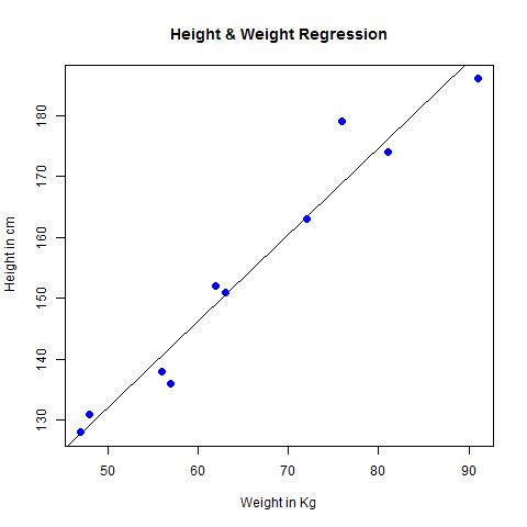
以圖形方式視覺化迴歸

線上演示

# Create the predictor and response variable.
x <- c(151, 174, 138, 186, 128, 136, 179, 163, 152, 131)
y <- c(63, 81, 56, 91, 47, 57, 76, 72, 62, 48)
relation <- lm(y~x)

# Give the chart file a name.
png(file = "linearregression.png")

# Plot the chart.
plot(y,x,col = "blue",main = "Height & Weight Regression",
abline(lm(x~y)),cex = 1.3,pch = 16,xlab = "Weight in Kg",ylab = "Height in cm")

# Save the file.
dev.off()

執行以上程式碼時，會產生以下結果：

列印頁面