Transformer中的多頭注意力機制

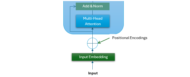
位置編碼是Transformer架構中一個至關重要的組成部分。位置編碼的輸出進入Transformer架構的第一個子層。這個子層是一個多頭注意力機制。

多頭注意力機制是Transformer模型的一個關鍵特性，它幫助模型更有效地處理順序資料。它允許模型同時檢視輸入序列的不同部分。

在本章中，我們將探討多頭注意力機制的結構、優點和Python實現。

什麼是自注意力機制？

自注意力機制，也稱為縮放點積注意力，是基於Transformer的模型的一個重要組成部分。它允許模型關注輸入序列中彼此相關的不同標記。這是透過計算輸入值的加權和來實現的。這裡的權重基於標記之間的相似性。

自注意力機制

以下是自注意力機制涉及的步驟：

建立查詢、鍵和值 - 自注意力機制將輸入序列中的每個標記轉換為三個向量，即查詢 (Q)、鍵 (K) 和值 (V)。
計算注意力分數 - 接下來，自注意力機制透過獲取查詢 (Q) 和鍵 (K) 矩陣的點積來計算注意力分數。注意力分數顯示每個單詞對當前正在處理的單詞的重要性。
應用Softmax函式 - 在此步驟中，應用Softmax函式將這些注意力分數轉換為機率，這確保注意力權重之和為1。
值的加權和 - 在最後一步中，使用Softmax注意力分數來計算值向量的加權和以產生輸出。

在數學上，自注意力機制可以用以下等式概括：

$$\mathrm{Self-Attention(Q,K,V) \: = \: softmax \left(\frac{QK^{T}}{\sqrt{d_{k}}}\right)V}$$

什麼是多頭注意力？

多頭注意力擴充套件了自注意力機制的概念，允許模型同時關注輸入序列的不同部分。多頭注意力不是執行單個注意力函式，而是並行執行多個自注意力機制或“頭”。這種方法使模型能夠更好地理解輸入序列中的各種關係和依賴關係。

請檢視下圖，它是原始Transformer架構的一部分。它代表了多頭子層的結構。

多頭注意力的步驟

以下是多頭注意力機制中涉及的關鍵步驟：

應用多個頭 - 首先，輸入嵌入被線性投影到多個查詢 (Q)、鍵 (K) 和值 (V) 矩陣集中（每個頭一個集合）。
執行並行自注意力 - 接下來，每個頭在其各自的投影上並行執行自注意力機制。
連線 - 現在，所有頭的輸出被連線起來。
組合資訊 - 在最後一步中，組合來自所有頭的資訊。這是透過將連線的輸出傳遞到最終的線性層來完成的。

在數學上，多頭注意力機制可以用以下等式概括：

$$\mathrm{MultiHead(Q,K,V) \: = \: Concat(head_{1}, \: \dotso \: ,head_{h})W^{\circ}}$$

其中每個頭計算如下：

$$\mathrm{head_{i}\:=\: Attention(QW_{i}^{Q}, \: KW_{i}^{K}, \: VW_{i}^{V} )\:=\: softmax\left(\frac{QW_{i}^{Q} (KW_{i}^{K})^{T}}{\sqrt{d_{k}}}\right)VW_{i}^{V}}$$

多頭注意力的優點

增強的表示 - 透過同時關注輸入序列的不同部分，多頭注意力使模型能夠更好地理解輸入序列中的各種關係和依賴關係。

並行處理 - 透過啟用並行處理，與RNN等順序模型相比，多頭注意力機制顯著提高了模型訓練效率。

示例

以下Python指令碼將實現多頭注意力機制。

import numpy as np

class MultiHeadAttention:
   def __init__(self, d_model, num_heads):
      self.d_model = d_model
      self.num_heads = num_heads
      assert d_model % num_heads == 0
      self.depth = d_model // num_heads

      # Initializing weight matrices for queries, keys, and values
      self.W_q = np.random.randn(d_model, d_model) * np.sqrt(2 / d_model)
      self.W_k = np.random.randn(d_model, d_model) * np.sqrt(2 / d_model)
      self.W_v = np.random.randn(d_model, d_model) * np.sqrt(2 / d_model)

      # Initializing weight matrix for output
      self.W_o = np.random.randn(d_model, d_model) * np.sqrt(2 / d_model)
        
   def split_heads(self, x, batch_size):
      """
      Split the last dimension into (num_heads, depth).
      Transpose the result to shape (batch_size, num_heads, seq_len, depth)
      """
      x = np.reshape(x, (batch_size, -1, self.num_heads, self.depth))
      return np.transpose(x, (0, 2, 1, 3))
    
   def scaled_dot_product_attention(self, q, k, v):
      """
      Compute scaled dot product attention.
      """
      matmul_qk = np.matmul(q, k)
      scaled_attention_logits = matmul_qk / np.sqrt(self.depth)
      scaled_attention_logits -= np.max(scaled_attention_logits, axis=-1, keepdims=True)
      attention_weights = np.exp(scaled_attention_logits)
      attention_weights /= np.sum(attention_weights, axis=-1, keepdims=True)
      output = np.matmul(attention_weights, v)
      return output, attention_weights
    
   def call(self, inputs):
      q, k, v = inputs
      batch_size = q.shape[0]

      # The Linear transformations
      q = np.dot(q, self.W_q)
      k = np.dot(k, self.W_k)
      v = np.dot(v, self.W_v)

      # Split heads
      q = self.split_heads(q, batch_size)
      k = self.split_heads(k, batch_size)
      v = self.split_heads(v, batch_size)

      # The Scaled dot-product attention
      attention_output, attention_weights = self.scaled_dot_product_attention(q, k.transpose(0, 1, 3, 2), v)

      # Combining heads
      attention_output = np.transpose(attention_output, (0, 2, 1, 3))
      concat_attention = np.reshape(attention_output, (batch_size, -1, self.d_model))

      # Linear transformation for output
      output = np.dot(concat_attention, self.W_o)

      return output, attention_weights

# An Example usage
d_model = 512
num_heads = 8
batch_size = 2
seq_len = 10

# Creating an instance of MultiHeadAttention
multi_head_attn = MultiHeadAttention(d_model, num_heads)

# Example input (batch_size, sequence_length, embedding_dim)
Q = np.random.randn(batch_size, seq_len, d_model)
K = np.random.randn(batch_size, seq_len, d_model)
V = np.random.randn(batch_size, seq_len, d_model)

# Performing multi-head attention
output, attention_weights = multi_head_attn.call([Q, K, V])

print("Input Query (Q):\n", Q)
print("Multi-Head Attention Output:\n", output)

輸出

實現上述指令碼後，我們將得到以下輸出。

Input Query (Q):
 [[[ 1.38223113 -0.41160481  1.00938637 ... -0.23466982 -0.20555623  0.80305284]
  [ 0.64676968 -0.83592083  2.45028238 ... -0.1884722  -0.25315478   0.18875416]
  [-0.52094419 -0.03697595 -0.61598294 ...  1.25611974 -0.35473911   0.15091853]
  ...
  [ 1.15939786 -0.5304271  -0.45396363 ...  0.8034571   0.66646109  -1.28586743]
  [ 0.6622964  -0.62871864  0.61371113 ... -0.59802729 -0.66135327  -0.24437055]
  [ 0.83111283 -0.81060387 -0.30858598 ... -0.74773536 -1.3032037   3.06236077]]

 [[-0.88579467 -0.15480352  0.76149486 ... -0.5033709   1.20498808  -0.55297549]
  [-1.11233207  0.7560376  -1.41004173 ... -2.12395203  2.15102493   0.09244935]
  [ 0.33003584  1.67364745 -0.30474183 ...  1.65907682 -0.61370707   0.58373516]
  ...
  [-2.07447136 -1.04964997 -0.15290381 ... -0.19912739 -1.02747937   0.20710549]
  [ 0.38910395 -1.04861089 -1.66583867 ...  0.21530474 -1.45005951   0.04472527]
  [-0.4718725  -0.45374148 -0.59990784 ... -1.9545574   0.11470969 1.03736175]]]

Multi-Head Attention Output:
 [[[ 0.36106079 -2.04297889  0.34937837 ...  0.11306262  0.53263072 -1.32641213]
  [ 1.09494311 -0.56658386  0.24210239 ...  1.1671274  -0.02322074   0.90110388]
  [ 0.45854972 -0.54493138 -0.63421376 ...  1.12479291  0.02585155  -0.08487499]
  ...
  [ 0.18252303 -0.17292067  0.46922657 ... -0.41311278 -1.17954406  -0.17005412]
  [-0.7849032  -2.12371221 -0.80403028 ... -2.35884088  0.15292393  -0.05569091]
  [ 1.07844261  0.18249226  0.81735183 ...  1.16346645 -1.71611237 -1.09860234]]

 [[ 0.58842816 -0.04493786 -1.72007093 ... -2.37506208 -1.83098896   2.84016717]
  [ 0.36608434  0.11709812  0.79108595 ... -1.6308595  -0.96052828   0.40893208]
  [-1.42113667  0.67459219 -0.8731377  ... -1.47390056 -0.42947079   1.04828361]
  ...
  [ 1.14151388 -1.5437165  -1.23405718 ...  0.29237056  0.56595327  -0.19385628]
  [-2.33028535  0.7245296   1.01725021 ... -0.9380485  -1.78988485   0.9938851 ]
  [-0.88115094  3.03051907  0.39447342 ... -1.89168756  0.94973626   0.61657539]
]]

結論

多頭注意力子層是Transformer架構的關鍵組成部分。它透過允許模型同時檢視輸入序列的不同部分來幫助模型更有效地處理順序資料。

在本章中，我們全面概述了多頭注意力機制、其優點以及如何使用Python實現它。

列印頁面