大資料分析 - 資料彙總

報告在大型資料分析中非常重要。每個組織都必須定期提供資訊來支援其決策過程。此任務通常由具有 SQL 和 ETL（提取、傳輸和載入）經驗的資料分析師處理。

負責此任務的團隊有責任將大資料分析部門產生的資訊傳播到組織的不同領域。

以下示例演示了資料彙總的含義。導航到資料夾bda/part1/summarize_data，並在資料夾內雙擊開啟summarize_data.Rproj檔案。然後，開啟summarize_data.R指令碼並檢視程式碼，並按照提供的說明進行操作。

# Install the following packages by running the following code in R. 
pkgs = c('data.table', 'ggplot2', 'nycflights13', 'reshape2') 
install.packages(pkgs)

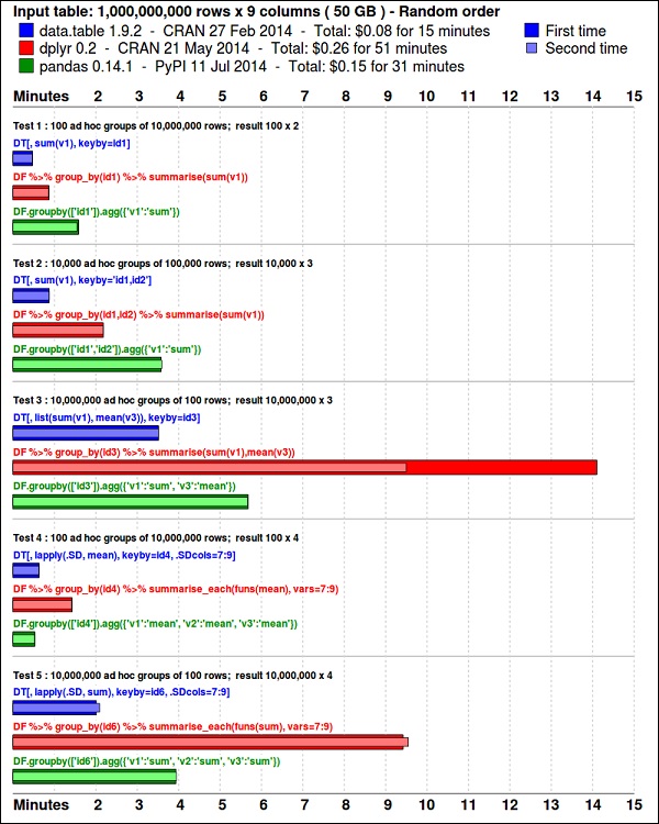
ggplot2包非常適合資料視覺化。data.table包是在R中進行快速且記憶體高效的彙總的絕佳選擇。最近的基準測試表明，它甚至比用於類似任務的 Python 庫pandas更快。

使用以下程式碼檢視資料。此程式碼也位於bda/part1/summarize_data/summarize_data.Rproj檔案中。

library(nycflights13) 
library(ggplot2) 
library(data.table) 
library(reshape2)  

# Convert the flights data.frame to a data.table object and call it DT 
DT <- as.data.table(flights)  

# The data has 336776 rows and 16 columns 
dim(DT)  

# Take a look at the first rows 
head(DT) 

#   year    month  day   dep_time  dep_delay  arr_time  arr_delay  carrier 
# 1: 2013     1     1      517       2         830         11       UA 
# 2: 2013     1     1      533       4         850         20       UA 
# 3: 2013     1     1      542       2         923         33       AA 
# 4: 2013     1     1      544      -1        1004        -18       B6 
# 5: 2013     1     1      554      -6         812        -25       DL 
# 6: 2013     1     1      554      -4         740         12       UA  

#     tailnum  flight  origin   dest    air_time   distance    hour   minute 
# 1:  N14228   1545     EWR      IAH      227        1400       5       17 
# 2:  N24211   1714     LGA      IAH      227        1416       5       33 
# 3:  N619AA   1141     JFK      MIA      160        1089       5       42 
# 4:  N804JB    725     JFK      BQN      183        1576       5       44 
# 5:  N668DN    461     LGA      ATL      116        762        5       54 
# 6:  N39463   1696     EWR      ORD      150        719        5       54

以下程式碼包含資料彙總的示例。

### Data Summarization
# Compute the mean arrival delay  
DT[, list(mean_arrival_delay = mean(arr_delay, na.rm = TRUE))] 
#        mean_arrival_delay 
# 1:           6.895377  
# Now, we compute the same value but for each carrier 
mean1 = DT[, list(mean_arrival_delay = mean(arr_delay, na.rm = TRUE)), 
   by = carrier] 
print(mean1) 
#      carrier    mean_arrival_delay 
# 1:      UA          3.5580111 
# 2:      AA          0.3642909 
# 3:      B6          9.4579733 
# 4:      DL          1.6443409 
# 5:      EV         15.7964311 
# 6:      MQ         10.7747334 
# 7:      US          2.1295951 
# 8:      WN          9.6491199 
# 9:      VX          1.7644644 
# 10:     FL         20.1159055 
# 11:     AS         -9.9308886 
# 12:     9E          7.3796692
# 13:     F9         21.9207048 
# 14:     HA         -6.9152047 
# 15:     YV         15.5569853 
# 16:     OO         11.9310345

# Now let’s compute to means in the same line of code 
mean2 = DT[, list(mean_departure_delay = mean(dep_delay, na.rm = TRUE), 
   mean_arrival_delay = mean(arr_delay, na.rm = TRUE)), 
   by = carrier] 
print(mean2) 

#       carrier    mean_departure_delay   mean_arrival_delay 
# 1:      UA            12.106073          3.5580111 
# 2:      AA             8.586016          0.3642909 
# 3:      B6            13.022522          9.4579733 
# 4:      DL             9.264505          1.6443409 
# 5:      EV            19.955390         15.7964311 
# 6:      MQ            10.552041         10.7747334 
# 7:      US             3.782418          2.1295951 
# 8:      WN            17.711744          9.6491199 
# 9:      VX            12.869421          1.7644644 
# 10:     FL            18.726075         20.1159055 
# 11:     AS             5.804775         -9.9308886 
# 12:     9E            16.725769          7.3796692 
# 13:     F9            20.215543         21.9207048 
# 14:     HA             4.900585         -6.9152047 
# 15:     YV            18.996330         15.5569853 
# 16:     OO            12.586207         11.9310345

### Create a new variable called gain 
# this is the difference between arrival delay and departure delay 
DT[, gain:= arr_delay - dep_delay]  

# Compute the median gain per carrier 
median_gain = DT[, median(gain, na.rm = TRUE), by = carrier] 
print(median_gain)