- 大資料分析教程
- 大資料分析 - 首頁
- 大資料分析 - 概述
- 大資料分析 - 特性
- 大資料分析 - 資料生命週期
- 大資料分析 - 架構
- 大資料分析 - 方法論
- 大資料分析 - 核心交付成果
- 大資料採用與規劃考慮
- 大資料分析 - 主要利益相關者
- 大資料分析 - 資料分析師
- 大資料分析 - 資料科學家
- 大資料分析有用資源
- 大資料分析 - 快速指南
- 大資料分析 - 資源
- 大資料分析 - 討論
大資料分析 - 統計方法
在分析資料時,可以使用統計方法。執行基本分析所需的常用工具包括:
- 相關性分析
- 方差分析
- 假設檢驗
處理大型資料集時,這些方法不會造成問題,因為除了相關性分析外,這些方法在計算上並不密集。在這種情況下,始終可以抽取樣本,結果應該穩健。
相關性分析
相關性分析旨在尋找數值變數之間的線性關係。這在不同情況下都很有用。一種常見用途是探索性資料分析,書中16.0.2節有一個這種方法的基本示例。首先,上述示例中使用的相關性指標基於**皮爾遜係數**。然而,還有一個有趣的相關性指標不受異常值的影響。這個指標稱為斯皮爾曼相關性。
**斯皮爾曼相關性**指標比皮爾遜方法更能抵抗異常值的影響,並且在資料不服從正態分佈時,能更好地估計數值變數之間的線性關係。
library(ggplot2)
# Select variables that are interesting to compare pearson and spearman
correlation methods.
x = diamonds[, c('x', 'y', 'z', 'price')]
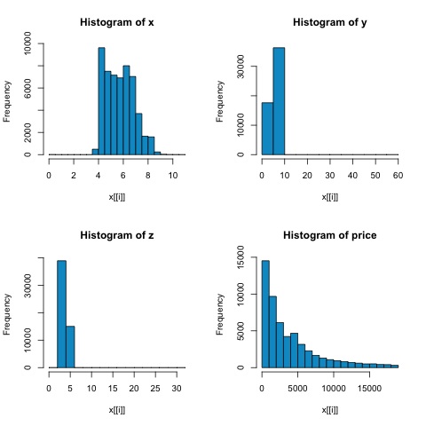
# From the histograms we can expect differences in the correlations of both
metrics.
# In this case as the variables are clearly not normally distributed, the
spearman correlation
# is a better estimate of the linear relation among numeric variables.
par(mfrow = c(2,2))
colnm = names(x)
for(i in 1:4) {
hist(x[[i]], col = 'deepskyblue3', main = sprintf('Histogram of %s', colnm[i]))
}
par(mfrow = c(1,1))
從下圖中的直方圖可以看出,兩種指標的相關性存在差異。在這種情況下,由於變數顯然不服從正態分佈,因此斯皮爾曼相關性是數值變數之間線性關係的更好估計。
為了在R中計算相關性,請開啟包含此程式碼部分的檔案**bda/part2/statistical_methods/correlation/correlation.R**。
## Correlation Matrix - Pearson and spearman
cor_pearson <- cor(x, method = 'pearson')
cor_spearman <- cor(x, method = 'spearman')

### Pearson Correlation
print(cor_pearson)
#            x          y          z        price
# x      1.0000000  0.9747015  0.9707718  0.8844352
# y      0.9747015  1.0000000  0.9520057  0.8654209
# z      0.9707718  0.9520057  1.0000000  0.8612494
# price  0.8844352  0.8654209  0.8612494  1.0000000

### Spearman Correlation
print(cor_spearman)
#              x          y          z      price
# x      1.0000000  0.9978949  0.9873553  0.9631961
# y      0.9978949  1.0000000  0.9870675  0.9627188
# z      0.9873553  0.9870675  1.0000000  0.9572323
# price  0.9631961  0.9627188  0.9572323  1.0000000
卡方檢驗
卡方檢驗允許我們檢驗兩個隨機變數是否獨立。這意味著每個變數的機率分佈都不會影響另一個變數。為了在R中評估檢驗,我們首先需要建立一個列聯表,然後將該表傳遞給**chisq.test R**函式。
例如,讓我們檢查diamonds資料集中的cut和color變數之間是否存在關聯。該檢驗正式定義為:
- H0:變數cut和diamond是獨立的
- H1:變數cut和diamond不是獨立的
從變數名稱來看,我們假設這兩個變數之間存在關係,但檢驗可以提供一個客觀的“規則”,說明此結果是否顯著。
在下面的程式碼片段中,我們發現檢驗的p值為2.2e-16,實際上幾乎為零。然後在進行**蒙特卡羅模擬**後執行檢驗,我們發現p值為0.0004998,仍然遠低於閾值0.05。此結果意味著我們拒絕零假設(H0),因此我們認為變數**cut**和**color**不是獨立的。
library(ggplot2)

# Use the table function to compute the contingency table
tbl = table(diamonds$cut, diamonds$color)
tbl

#              D    E    F    G    H    I    J
# Fair       163  224  312  314  303  175  119
# Good       662  933  909  871  702  522  307
# Very Good 1513 2400 2164 2299 1824 1204  678
# Premium   1603 2337 2331 2924 2360 1428  808
# Ideal     2834 3903 3826 4884 3115 2093  896

# In order to run the test we just use the chisq.test function.
chisq.test(tbl)

# Pearson’s Chi-squared test
# data:  tbl
# X-squared = 310.32, df = 24, p-value < 2.2e-16
# It is also possible to compute the p-values using a monte-carlo simulation
# It's needed to add the simulate.p.value = TRUE flag and the amount of
simulations
chisq.test(tbl, simulate.p.value = TRUE, B = 2000)

# Pearson’s Chi-squared test with simulated p-value (based on 2000 replicates)
# data:  tbl
# X-squared = 310.32, df = NA, p-value = 0.0004998
t檢驗
**t檢驗**的目的是評估名義變數的不同組之間數值變數的分佈是否存在差異。為了演示這一點,我將選擇因子變數cut的Fair和Ideal水平,然後我們將比較這兩個組之間數值變數的值。
data = diamonds[diamonds$cut %in% c('Fair', 'Ideal'), ]

data$cut = droplevels.factor(data$cut) # Drop levels that aren’t used from the
cut variable
df1 = data[, c('cut', 'price')]

# We can see the price means are different for each group
tapply(df1$price, df1$cut, mean)
# Fair    Ideal
# 4358.758 3457.542
t檢驗在R中使用**t.test**函式實現。t.test的公式介面是最簡單的使用方法,其思想是用組變數解釋數值變數。
例如:**t.test(numeric_variable ~ group_variable, data = data)**。在前面的示例中,**numeric_variable**是**price**,**group_variable**是**cut**。
從統計學的角度來看,我們正在檢驗數值變數在兩組之間的分佈是否存在差異。正式的假設檢驗用零假設(H0)和備擇假設(H1)來描述。
H0:Fair和Ideal組之間price變數的分佈沒有差異
H1:Fair和Ideal組之間price變數的分佈存在差異
以下可以在R中使用以下程式碼實現:
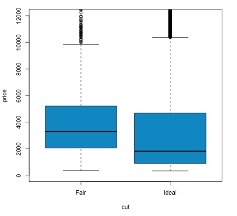
t.test(price ~ cut, data = data)

# Welch Two Sample t-test
#
# data:  price by cut
# t = 9.7484, df = 1894.8, p-value < 2.2e-16
# alternative hypothesis: true difference in means is not equal to 0
# 95 percent confidence interval:
#   719.9065 1082.5251
# sample estimates:
#   mean in group Fair mean in group Ideal
#   4358.758            3457.542

# Another way to validate the previous results is to just plot the
distributions using a box-plot
plot(price ~ cut, data = data, ylim = c(0,12000),
   col = 'deepskyblue3')
我們可以透過檢查p值是否小於0.05來分析檢驗結果。如果是這種情況,我們保留備擇假設。這意味著我們在cut因子的兩個水平之間發現了價格差異。從水平的名稱來看,我們本可以預期這個結果,但我們不會預期Fail組的平均價格會高於Ideal組。我們可以透過比較每個因子的均值來觀察這一點。
**plot**命令生成的圖形顯示了價格和cut變數之間的關係。這是一個箱線圖;我們在16.0.1節中介紹過這種圖,但它基本上顯示了我們正在分析的cut的兩個水平的price變數的分佈。
方差分析
方差分析(ANOVA)是一種統計模型,用於透過比較每組的均值和方差來分析組分佈之間的差異,該模型由羅納德·費舍爾開發。ANOVA提供了一個統計檢驗,用於檢驗多個組的均值是否相等,因此它將t檢驗推廣到多於兩組的情況。
ANOVA對於比較三個或更多組的統計顯著性很有用,因為進行多次雙樣本t檢驗會導致犯I型統計錯誤的可能性增加。
在提供數學解釋方面,需要了解以下內容才能理解該檢驗。
xij = x + (xi − x) + (xij − x)
這導致以下模型:
xij = μ + αi + ∈ij
其中μ是總均值,αi是第i個組均值。誤差項∈ij假設來自正態分佈的iid。檢驗的零假設是:
α1 = α2 = … = αk
在計算檢驗統計量方面,我們需要計算兩個值:
- 組間差異的平方和:
$$SSD_B = \sum_{i}^{k} \sum_{j}^{n}(\bar{x_{\bar{i}}} - \bar{x})^2$$
- 組內平方和
$$SSD_W = \sum_{i}^{k} \sum_{j}^{n}(\bar{x_{\bar{ij}}} - \bar{x_{\bar{i}}})^2$$
其中SSDB的自由度為k−1,SSDW的自由度為N−k。然後我們可以定義每個指標的均方差。
MSB = SSDB / (k - 1)
MSw = SSDw / (N - k)
最後,ANOVA中的檢驗統計量定義為上述兩個量的比率
F = MSB / MSw
它服從自由度為k−1和N−k的F分佈。如果零假設為真,F值可能接近1。否則,組間均方MSB可能很大,這將導致較大的F值。
基本上,ANOVA檢查總方差的兩個來源,並檢視哪個部分的貢獻更大。這就是為什麼它被稱為方差分析,儘管目的是比較組均值。
在計算統計量方面,在R中實際上相當簡單。以下示例將演示如何操作以及如何繪製結果。
library(ggplot2)
# We will be using the mtcars dataset

head(mtcars)
#                    mpg  cyl disp  hp drat  wt  qsec   vs am  gear carb
# Mazda RX4         21.0   6  160 110 3.90 2.620 16.46  0  1    4    4
# Mazda RX4 Wag     21.0   6  160 110 3.90 2.875 17.02  0  1    4    4
# Datsun 710        22.8   4  108  93 3.85 2.320 18.61  1  1    4    1
# Hornet 4 Drive    21.4   6  258 110 3.08 3.215 19.44  1  0    3    1
# Hornet Sportabout 18.7   8  360 175 3.15 3.440 17.02  0  0    3    2
# Valiant           18.1   6  225 105 2.76 3.460 20.22  1  0    3    1

# Let's see if there are differences between the groups of cyl in the mpg variable.
data = mtcars[, c('mpg', 'cyl')]
fit = lm(mpg ~ cyl, data = mtcars)
anova(fit)

# Analysis of Variance Table
# Response: mpg
#           Df Sum Sq Mean Sq F value    Pr(>F)
# cyl        1 817.71  817.71  79.561 6.113e-10 ***
# Residuals 30 308.33   10.28
# Signif. codes:  0 *** 0.001 ** 0.01 * 0.05 .
# Plot the distribution
plot(mpg ~ as.factor(cyl), data = mtcars, col = 'deepskyblue3')
程式碼將產生以下輸出:
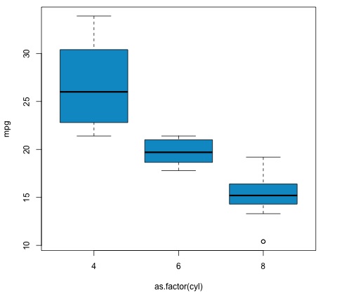
我們在示例中獲得的p值遠小於0.05,因此R返回符號'***'來表示這一點。這意味著我們拒絕零假設,並且我們在cyl變數的不同組之間發現了mpg均值的差異。