SciPy - integrate.romb() 方法

SciPy integrate.romb() 方法用於執行數值積分或羅姆伯格積分任務。此方法還幫助我們根據樣本/座標點繪製圖形。

語法

以下為 SciPy integrate.romb() 方法的語法 -

romb(y, dx = int_val/float_val/1.0)

引數

此函式接受以下引數 -

• y: 此引數確定離散點上的陣列函式，並且這些點被認為是均勻間隔開的。
• dx: 此引數確定點之間的間隔，如果未指定，其預設值為 1.0。

返回值

此方法返回型別為浮點數的估計值。

示例 1

以下為展示簡單的積分函式 SciPy integrate.romb() 方法，即 f(x) = x²，其中積分割槽間在 0 到 1 之間。最終值基於五個離散點。

import numpy as np
from scipy import integrate

# define the function values at discrete points
x = np.linspace(0, 1, 5)
y = x**2 

# calculate the integral
res_integral = integrate.romb(y, dx=x[1] - x[0])

# display the result
print(res_integral)

輸出

以上程式碼產生以下結果 -

0.3333333333333333

示例 2

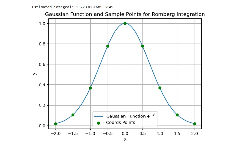
這個程式演示了高斯函式（即 e^-x2）在 -2 到 2 之間區間的數值積分，並且該函式值被表示為九個點（x 軸）。

import numpy as np
from scipy.integrate import romb
import matplotlib.pyplot as plt

# define the function values at discrete points
x = np.linspace(-2, 2, 9)
y = np.exp(-x**2)

# calculate the integral
res_integral = romb(y, dx=x[1] - x[0])

# display the result
print(f"Estimated integral: {res_integral}")

# plot the Gaussian function and the points used in Romberg integration
x_fine = np.linspace(-2, 2, 1000)
y_fine = np.exp(-x_fine**2)

plt.plot(x_fine, y_fine, label='Gaussian Function $e^{-x^2}$')
plt.scatter(x, y, color='green', zorder=5, label='coords Points')

plt.title('Gaussian Function and Sample Points for Romberg Integration')
plt.xlabel('x')
plt.ylabel('y')
plt.legend()
plt.grid(True)
plt.show()

輸出

以上程式碼產生以下結果 -