- Python Pandas 教程
- Python Pandas - 首頁
- Python Pandas - 簡介
- Python Pandas - 環境設定
- Python Pandas - 基礎知識
- Python Pandas - 資料結構介紹
- Python Pandas - 索引物件
- Python Pandas - Panel
- Python Pandas - 基本功能
- Python Pandas - 索引和資料選擇
- Python Pandas - Series
- Python Pandas - Series
- Python Pandas - 切片 Series 物件
- Python Pandas - Series 物件的屬性
- Python Pandas - Series 物件的算術運算
- Python Pandas - 將 Series 轉換為其他物件
- Python Pandas - DataFrame
- Python Pandas - DataFrame
- Python Pandas - 訪問 DataFrame
- Python Pandas - 切片 DataFrame 物件
- Python Pandas - 修改 DataFrame
- Python Pandas - 從 DataFrame 中刪除行
- Python Pandas - DataFrame 的算術運算
- Python Pandas - I/O 工具
- Python Pandas - I/O 工具
- Python Pandas - 使用 CSV 格式
- Python Pandas - 讀取和寫入 JSON 檔案
- Python Pandas - 從 Excel 檔案讀取資料
- Python Pandas - 將資料寫入 Excel 檔案
- Python Pandas - 使用 HTML 資料
- Python Pandas - 剪貼簿
- Python Pandas - 使用 HDF5 格式
- Python Pandas - 與 SQL 的比較
- Python Pandas - 資料處理
- Python Pandas - 排序
- Python Pandas - 重新索引
- Python Pandas - 迭代
- Python Pandas - 級聯
- Python Pandas - 統計函式
- Python Pandas - 描述性統計
- Python Pandas - 使用文字資料
- Python Pandas - 函式應用
- Python Pandas - 選項和自定義
- Python Pandas - 視窗函式
- Python Pandas - 聚合
- Python Pandas - 合併/連線
- Python Pandas - 多層索引
- Python Pandas - 多層索引的基礎知識
- Python Pandas - 使用多層索引進行索引
- Python Pandas - 使用多層索引進行高階重新索引
- Python Pandas - 重新命名多層索引標籤
- Python Pandas - 對多層索引進行排序
- Python Pandas - 二元運算
- Python Pandas - 二元比較運算
- Python Pandas - 布林索引
- Python Pandas - 布林掩碼
- Python Pandas - 資料重塑和透視
- Python Pandas - 透視表
- Python Pandas - 堆疊和取消堆疊
- Python Pandas - 熔化
- Python Pandas - 計算虛擬變數
- Python Pandas - 分類資料
- Python Pandas - 分類資料
- Python Pandas - 分類資料的排序和排序
- Python Pandas - 比較分類資料
- Python Pandas - 處理缺失資料
- Python Pandas - 缺失資料
- Python Pandas - 填充缺失資料
- Python Pandas - 缺失值的插值
- Python Pandas - 刪除缺失資料
- Python Pandas - 使用缺失資料進行計算
- Python Pandas - 處理重複項
- Python Pandas - 重複資料
- Python Pandas - 計數和檢索唯一元素
- Python Pandas - 重複標籤
- Python Pandas - 分組和聚合
- Python Pandas - GroupBy
- Python Pandas - 時間序列資料
- Python Pandas - 日期功能
- Python Pandas - Timedelta
- Python Pandas - 稀疏資料結構
- Python Pandas - 稀疏資料
- Python Pandas - 視覺化
- Python Pandas - 視覺化
- Python Pandas - 附加概念
- Python Pandas - 警告和陷阱
- Python Pandas 有用資源
- Python Pandas 快速指南
- Python Pandas - 有用資源
- Python Pandas - 討論
Python Pandas 快速指南
Python Pandas - 簡介
Pandas 是一個開源的 Python 庫,它使用強大的資料結構提供高效能的資料操作和分析工具。Pandas 的名稱來源於面板資料——計量經濟學中的多維資料。
2008 年,開發者 Wes McKinney 在需要一個高效能、靈活的工具來分析資料時開始開發 pandas。
在 Pandas 之前,Python 主要用於資料清洗和準備。它對資料分析的貢獻非常小。Pandas解決了這個問題。使用 Pandas,我們可以完成資料處理和分析中的五個典型步驟,無論資料來源如何——載入、準備、操作、建模和分析。
Python 與 Pandas 廣泛應用於包括金融、經濟學、統計學、分析學等在內的學術和商業領域。
Pandas 的關鍵特性
- 快速高效的 DataFrame 物件,具有預設和自定義索引。
- 用於將資料從不同檔案格式載入到記憶體中資料物件的工具。
- 資料對齊和缺失資料的整合處理。
- 資料集的重塑和透視。
- 基於標籤的大型資料集的切片、索引和子集選擇。
- 可以刪除或插入資料結構中的列。
- 對資料進行分組以進行聚合和轉換。
- 高效能的資料合併和連線。
- 時間序列功能。
Python Pandas - 環境設定
標準 Python 發行版不包含 Pandas 模組。一個輕量級的替代方案是使用流行的 Python 包安裝程式 **pip** 安裝 NumPy。
pip install pandas
如果您安裝 Anaconda Python 包,Pandas 將預設安裝如下:
Windows
**Anaconda** (來自 https://www.continuum.io) 是一個免費的 SciPy 棧 Python 發行版。它也適用於 Linux 和 Mac。
**Canopy** (https://www.enthought.com/products/canopy/) 提供免費和商業發行版,包含適用於 Windows、Linux 和 Mac 的完整 SciPy 棧。
**Python(x,y)** 是一個免費的 Python 發行版,包含 SciPy 棧和 Spyder IDE,適用於 Windows 作業系統。(可從 http://python-xy.github.io/ 下載)
Linux
各個 Linux 發行版的包管理器用於安裝 SciPy 棧中的一個或多個包。
對於 Ubuntu 使用者
sudo apt-get install python-numpy python-scipy python-matplotlibipythonipythonnotebook
python-pandas python-sympy python-nose
對於 Fedora 使用者
sudo yum install numpyscipy python-matplotlibipython python-pandas sympy
python-nose atlas-devel
資料結構介紹
Pandas 處理以下三種資料結構:
- Series
- DataFrame
- Panel
這些資料結構構建在 Numpy 陣列之上,這意味著它們速度很快。
維度和描述
理解這些資料結構的最佳方法是,更高維的資料結構是其低維資料結構的容器。例如,DataFrame 是 Series 的容器,Panel 是 DataFrame 的容器。
| 資料結構 | 維度 | 描述 |
|---|---|---|
| Series | 1 | 一維帶標籤的同質陣列,大小不可變。 |
| DataFrame | 2 | 一般的二維帶標籤的、大小可變的表格結構,可能包含異構型別的列。 |
| Panel | 3 | 一般的三維帶標籤的、大小可變的陣列。 |
構建和處理兩個或多個維度的陣列是一項繁瑣的任務,使用者需要在編寫函式時考慮資料集的方向。但是使用 Pandas 資料結構,可以減少使用者的腦力負擔。
例如,對於表格資料 (DataFrame),從語義上講,考慮 **索引**(行)和 **列** 比考慮軸 0 和軸 1更有幫助。
可變性
所有 Pandas 資料結構的值都是可變的(可以更改),除了 Series 之外,所有資料結構的大小都是可變的。Series 的大小是不可變的。
**注意** - DataFrame 廣泛使用,並且是最重要的資料結構之一。Panel 的使用要少得多。
Series
Series 是一種一維類似陣列的結構,包含同質資料。例如,以下 Series 是整數 10、23、56……的集合。
| 10 | 23 | 56 | 17 | 52 | 61 | 73 | 90 | 26 | 72 |
關鍵點
- 同質資料
- 大小不可變
- 資料值可變
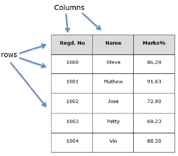
DataFrame
DataFrame 是一個二維陣列,包含異構資料。例如:
| 姓名 | 年齡 | 性別 | 評分 |
|---|---|---|---|
| Steve | 32 | 男 | 3.45 |
| Lia | 28 | 女 | 4.6 |
| Vin | 45 | 男 | 3.9 |
| Katie | 38 | 女 | 2.78 |
該表顯示了一個組織銷售團隊的資料及其整體績效評分。資料以行和列表示。每一列代表一個屬性,每一行代表一個人。
列的資料型別
四列的資料型別如下:
| 列 | 型別 |
|---|---|
| 姓名 | 字串 |
| 年齡 | 整數 |
| 性別 | 字串 |
| 評分 | 浮點數 |
關鍵點
- 異構資料
- 大小可變
- 資料可變
Panel
Panel 是一種三維資料結構,包含異構資料。很難用圖形表示來表示 Panel。但是,Panel 可以被說明為 DataFrame 的容器。
關鍵點
- 異構資料
- 大小可變
- 資料可變
Python Pandas - Series
Series 是一種一維帶標籤的陣列,能夠儲存任何型別的資料(整數、字串、浮點數、Python 物件等)。軸標籤統稱為索引。
pandas.Series
可以使用以下建構函式建立 pandas Series:
pandas.Series( data, index, dtype, copy)
建構函式的引數如下:
| 序號 | 引數和描述 |
|---|---|
| 1 |
data data 可以採用各種形式,例如 ndarray、列表、常量 |
| 2 |
index 索引值必須唯一且可雜湊,與 data 長度相同。如果沒有傳遞索引,則預設為 **np.arange(n)**。 |
| 3 |
dtype dtype 用於資料型別。如果為 None,則將推斷資料型別 |
| 4 |
copy 複製資料。預設為 False |
可以使用各種輸入建立 Series,例如:
- 陣列
- 字典
- 標量值或常量
建立空 Series
可以建立的基本 Series 是空 Series。
示例
#import the pandas library and aliasing as pd
import pandas as pd
s = pd.Series()
print s
其 **輸出** 如下:
Series([], dtype: float64)
從 ndarray 建立 Series
如果 data 是一個 ndarray,則傳遞的 index 必須具有相同的長度。如果沒有傳遞 index,則預設情況下 index 將為 **range(n)**,其中 **n** 是陣列長度,即 [0,1,2,3…. **range(len(array))-1]。**
示例 1
#import the pandas library and aliasing as pd
import pandas as pd
import numpy as np
data = np.array(['a','b','c','d'])
s = pd.Series(data)
print s
其 **輸出** 如下:
0   a
1   b
2   c
3   d
dtype: object
我們沒有傳遞任何 index,因此預設情況下,它分配了從 0 到 **len(data)-1** 的索引,即 0 到 3。
示例 2
#import the pandas library and aliasing as pd
import pandas as pd
import numpy as np
data = np.array(['a','b','c','d'])
s = pd.Series(data,index=[100,101,102,103])
print s
其 **輸出** 如下:
100  a
101  b
102  c
103  d
dtype: object
我們在這裡傳遞了 index 值。現在我們可以在輸出中看到自定義的索引值。
從字典建立 Series
可以將 **字典** 作為輸入傳遞,如果未指定 index,則字典鍵將按排序順序排列以構建 index。如果傳遞了 **index**,則將提取與 index 中標籤對應的 data 中的值。
示例 1
#import the pandas library and aliasing as pd
import pandas as pd
import numpy as np
data = {'a' : 0., 'b' : 1., 'c' : 2.}
s = pd.Series(data)
print s
其 **輸出** 如下:
a 0.0
b 1.0
c 2.0
dtype: float64
**注意** - 字典鍵用於構建索引。
示例 2
#import the pandas library and aliasing as pd
import pandas as pd
import numpy as np
data = {'a' : 0., 'b' : 1., 'c' : 2.}
s = pd.Series(data,index=['b','c','d','a'])
print s
其 **輸出** 如下:
b 1.0
c 2.0
d NaN
a 0.0
dtype: float64
**注意** - 保留索引順序,缺失元素用 NaN(非數字)填充。
從標量建立 Series
如果 data 是一個標量值,則必須提供 index。該值將重複以匹配 **index** 的長度
#import the pandas library and aliasing as pd
import pandas as pd
import numpy as np
s = pd.Series(5, index=[0, 1, 2, 3])
print s
其 **輸出** 如下:
0  5
1  5
2  5
3  5
dtype: int64
使用位置從 Series 訪問資料
序列中的資料可以像訪問ndarray一樣訪問。
示例 1
檢索第一個元素。我們已經知道,陣列的計數從零開始,這意味著第一個元素儲存在第零個位置,以此類推。
import pandas as pd
s = pd.Series([1,2,3,4,5],index = ['a','b','c','d','e'])

#retrieve the first element
print s[0]
其 **輸出** 如下:
1
示例 2
檢索序列中的前三個元素。如果在前面插入一個:,則將提取從該索引開始的所有項。如果使用兩個引數(它們之間用:隔開),則提取這兩個索引之間的項(不包括停止索引)。
import pandas as pd
s = pd.Series([1,2,3,4,5],index = ['a','b','c','d','e'])

#retrieve the first three element
print s[:3]
其 **輸出** 如下:
a  1
b  2
c  3
dtype: int64
示例3
檢索最後三個元素。
import pandas as pd
s = pd.Series([1,2,3,4,5],index = ['a','b','c','d','e'])

#retrieve the last three element
print s[-3:]
其 **輸出** 如下:
c  3
d  4
e  5
dtype: int64
使用標籤(索引)檢索資料
Series類似於固定大小的dict,您可以透過索引標籤獲取和設定值。
示例 1
使用索引標籤值檢索單個元素。
import pandas as pd
s = pd.Series([1,2,3,4,5],index = ['a','b','c','d','e'])

#retrieve a single element
print s['a']
其 **輸出** 如下:
1
示例 2
使用索引標籤值的列表檢索多個元素。
import pandas as pd
s = pd.Series([1,2,3,4,5],index = ['a','b','c','d','e'])

#retrieve multiple elements
print s[['a','c','d']]
其 **輸出** 如下:
a  1
c  3
d  4
dtype: int64
示例3
如果標籤不存在,則會引發異常。
import pandas as pd
s = pd.Series([1,2,3,4,5],index = ['a','b','c','d','e'])

#retrieve multiple elements
print s['f']
其 **輸出** 如下:
…
KeyError: 'f'
Python Pandas - DataFrame
DataFrame是一個二維資料結構,即資料以表格形式在行和列中對齊。
DataFrame的特徵
- 列的型別可能不同
- 大小——可變
- 帶標籤的軸(行和列)
- 可以對行和列執行算術運算
結構
讓我們假設我們正在建立一個包含學生資料的資料框。
您可以將其視為SQL表或電子表格資料表示。
pandas.DataFrame
可以使用以下建構函式建立pandas DataFrame:
pandas.DataFrame( data, index, columns, dtype, copy)
建構函式的引數如下:
| 序號 | 引數和描述 |
|---|---|
| 1 |
data data採用多種形式,例如ndarray、series、map、列表、dict、常量以及另一個DataFrame。 |
| 2 |
index 對於行標籤,用於結果框架的索引是可選的,如果沒有傳遞索引,則預設為np.arange(n)。 |
| 3 |
列 對於列標籤,可選的預設語法是- np.arange(n)。只有在沒有傳遞索引的情況下才為真。 |
| 4 |
dtype 每列的資料型別。 |
| 5 |
copy 此命令(或任何它是什麼)用於複製資料,如果預設值為False。 |
建立DataFrame
可以使用各種輸入建立pandas DataFrame,例如:
- 列表
- 字典
- Series
- NumPy ndarrays
- 另一個DataFrame
在本章的後續部分,我們將看到如何使用這些輸入建立DataFrame。
建立空DataFrame
可以建立的基本DataFrame是一個空DataFrame。
示例
#import the pandas library and aliasing as pd
import pandas as pd
df = pd.DataFrame()
print df
其 **輸出** 如下:
Empty DataFrame
Columns: []
Index: []
從列表建立DataFrame
可以使用單個列表或列表的列表建立DataFrame。
示例 1
import pandas as pd
data = [1,2,3,4,5]
df = pd.DataFrame(data)
print df
其 **輸出** 如下:
     0
0    1
1    2
2    3
3    4
4    5
示例 2
import pandas as pd
data = [['Alex',10],['Bob',12],['Clarke',13]]
df = pd.DataFrame(data,columns=['Name','Age'])
print df
其 **輸出** 如下:
      Name      Age
0     Alex      10
1     Bob       12
2     Clarke    13
示例3
import pandas as pd
data = [['Alex',10],['Bob',12],['Clarke',13]]
df = pd.DataFrame(data,columns=['Name','Age'],dtype=float)
print df
其 **輸出** 如下:
      Name     Age
0     Alex     10.0
1     Bob      12.0
2     Clarke   13.0
注意——觀察,dtype引數將“年齡”列的型別更改為浮點型。
從ndarray/列表的字典建立DataFrame
所有ndarrays的長度必須相同。如果傳遞了索引,則索引的長度應等於陣列的長度。
如果沒有傳遞索引,則預設情況下,索引將為range(n),其中n為陣列長度。
示例 1
import pandas as pd
data = {'Name':['Tom', 'Jack', 'Steve', 'Ricky'],'Age':[28,34,29,42]}
df = pd.DataFrame(data)
print df
其 **輸出** 如下:
      Age      Name
0     28        Tom
1     34       Jack
2     29      Steve
3     42      Ricky
注意——觀察值0,1,2,3。它們是使用函式range(n)為每個值分配的預設索引。
示例 2
現在讓我們使用陣列建立一個帶索引的DataFrame。
import pandas as pd
data = {'Name':['Tom', 'Jack', 'Steve', 'Ricky'],'Age':[28,34,29,42]}
df = pd.DataFrame(data, index=['rank1','rank2','rank3','rank4'])
print df
其 **輸出** 如下:
         Age    Name
rank1    28      Tom
rank2    34     Jack
rank3    29    Steve
rank4    42    Ricky
注意——觀察,index引數為每一行分配一個索引。
從字典列表建立DataFrame
字典列表可以作為輸入資料傳遞來建立DataFrame。字典鍵預設作為列名。
示例 1
以下示例演示如何透過傳遞字典列表來建立DataFrame。
import pandas as pd
data = [{'a': 1, 'b': 2},{'a': 5, 'b': 10, 'c': 20}]
df = pd.DataFrame(data)
print df
其 **輸出** 如下:
    a    b      c
0   1   2     NaN
1   5   10   20.0
注意——觀察,NaN(非數字)附加在缺失區域。
示例 2
以下示例演示如何透過傳遞字典列表和行索引來建立DataFrame。
import pandas as pd
data = [{'a': 1, 'b': 2},{'a': 5, 'b': 10, 'c': 20}]
df = pd.DataFrame(data, index=['first', 'second'])
print df
其 **輸出** 如下:
        a   b       c
first   1   2     NaN
second  5   10   20.0
示例3
以下示例演示如何使用字典列表、行索引和列索引建立DataFrame。
import pandas as pd
data = [{'a': 1, 'b': 2},{'a': 5, 'b': 10, 'c': 20}]

#With two column indices, values same as dictionary keys
df1 = pd.DataFrame(data, index=['first', 'second'], columns=['a', 'b'])

#With two column indices with one index with other name
df2 = pd.DataFrame(data, index=['first', 'second'], columns=['a', 'b1'])
print df1
print df2
其 **輸出** 如下:
#df1 output
         a  b
first    1  2
second   5  10

#df2 output
         a  b1
first    1  NaN
second   5  NaN
注意——觀察,df2 DataFrame是用字典鍵以外的列索引建立的;因此,在適當的位置附加了NaN。而df1是用與字典鍵相同的列索引建立的,因此附加了NaN。
從Series的字典建立DataFrame
可以傳遞Series的字典來形成DataFrame。結果索引是傳遞的所有Series索引的並集。
示例
import pandas as pd

d = {'one' : pd.Series([1, 2, 3], index=['a', 'b', 'c']),
   'two' : pd.Series([1, 2, 3, 4], index=['a', 'b', 'c', 'd'])}

df = pd.DataFrame(d)
print df
其 **輸出** 如下:
      one    two
a     1.0    1
b     2.0    2
c     3.0    3
d     NaN    4
注意——觀察,對於series one,沒有傳遞標籤‘d’,但在結果中,對於d標籤,附加了NaN。
現在讓我們透過示例瞭解列選擇、新增和刪除。
列選擇
我們將透過從DataFrame中選擇一列來理解這一點。
示例
import pandas as pd

d = {'one' : pd.Series([1, 2, 3], index=['a', 'b', 'c']),
   'two' : pd.Series([1, 2, 3, 4], index=['a', 'b', 'c', 'd'])}

df = pd.DataFrame(d)
print df ['one']
其 **輸出** 如下:
a     1.0
b     2.0
c     3.0
d     NaN
Name: one, dtype: float64
列新增
我們將透過向現有資料框新增新列來理解這一點。
示例
import pandas as pd

d = {'one' : pd.Series([1, 2, 3], index=['a', 'b', 'c']),
   'two' : pd.Series([1, 2, 3, 4], index=['a', 'b', 'c', 'd'])}

df = pd.DataFrame(d)

# Adding a new column to an existing DataFrame object with column label by passing new series

print ("Adding a new column by passing as Series:")
df['three']=pd.Series([10,20,30],index=['a','b','c'])
print df

print ("Adding a new column using the existing columns in DataFrame:")
df['four']=df['one']+df['three']

print df
其 **輸出** 如下:
Adding a new column by passing as Series:
     one   two   three
a    1.0    1    10.0
b    2.0    2    20.0
c    3.0    3    30.0
d    NaN    4    NaN

Adding a new column using the existing columns in DataFrame:
      one   two   three    four
a     1.0    1    10.0     11.0
b     2.0    2    20.0     22.0
c     3.0    3    30.0     33.0
d     NaN    4     NaN     NaN
列刪除
列可以被刪除或彈出;讓我們舉個例子來理解如何操作。
示例
# Using the previous DataFrame, we will delete a column
# using del function
import pandas as pd

d = {'one' : pd.Series([1, 2, 3], index=['a', 'b', 'c']),
   'two' : pd.Series([1, 2, 3, 4], index=['a', 'b', 'c', 'd']),
   'three' : pd.Series([10,20,30], index=['a','b','c'])}

df = pd.DataFrame(d)
print ("Our dataframe is:")
print df

# using del function
print ("Deleting the first column using DEL function:")
del df['one']
print df

# using pop function
print ("Deleting another column using POP function:")
df.pop('two')
print df
其 **輸出** 如下:
Our dataframe is:
      one   three  two
a     1.0    10.0   1
b     2.0    20.0   2
c     3.0    30.0   3
d     NaN     NaN   4

Deleting the first column using DEL function:
      three    two
a     10.0     1
b     20.0     2
c     30.0     3
d     NaN      4

Deleting another column using POP function:
   three
a  10.0
b  20.0
c  30.0
d  NaN
行選擇、新增和刪除
我們現在將透過示例瞭解行選擇、新增和刪除。讓我們從選擇的概念開始。
按標籤選擇
可以透過將行標籤傳遞給loc函式來選擇行。
import pandas as pd

d = {'one' : pd.Series([1, 2, 3], index=['a', 'b', 'c']),
   'two' : pd.Series([1, 2, 3, 4], index=['a', 'b', 'c', 'd'])}

df = pd.DataFrame(d)
print df.loc['b']
其 **輸出** 如下:
one 2.0
two 2.0
Name: b, dtype: float64
結果是一個系列,其標籤作為DataFrame的列名。並且,該系列的名稱是檢索它的標籤。
按整數位置選擇
可以透過將整數位置傳遞給iloc函式來選擇行。
import pandas as pd

d = {'one' : pd.Series([1, 2, 3], index=['a', 'b', 'c']),
   'two' : pd.Series([1, 2, 3, 4], index=['a', 'b', 'c', 'd'])}

df = pd.DataFrame(d)
print df.iloc[2]
其 **輸出** 如下:
one   3.0
two   3.0
Name: c, dtype: float64
切片行
可以使用“:”運算子選擇多行。
import pandas as pd

d = {'one' : pd.Series([1, 2, 3], index=['a', 'b', 'c']),
   'two' : pd.Series([1, 2, 3, 4], index=['a', 'b', 'c', 'd'])}

df = pd.DataFrame(d)
print df[2:4]
其 **輸出** 如下:
   one  two
c  3.0    3
d  NaN    4
新增行
使用append函式將新行新增到DataFrame。此函式將在末尾附加行。
import pandas as pd

df = pd.DataFrame([[1, 2], [3, 4]], columns = ['a','b'])
df2 = pd.DataFrame([[5, 6], [7, 8]], columns = ['a','b'])

df = df.append(df2)
print df
其 **輸出** 如下:
   a  b
0  1  2
1  3  4
0  5  6
1  7  8
刪除行
使用索引標籤從DataFrame中刪除或刪除行。如果標籤重複,則將刪除多行。
如果您觀察到,在上例中,標籤是重複的。讓我們刪除一個標籤,看看將刪除多少行。
import pandas as pd

df = pd.DataFrame([[1, 2], [3, 4]], columns = ['a','b'])
df2 = pd.DataFrame([[5, 6], [7, 8]], columns = ['a','b'])

df = df.append(df2)

# Drop rows with label 0
df = df.drop(0)

print df
其 **輸出** 如下:
  a b
1 3 4
1 7 8
在上例中,刪除了兩行,因為這兩行包含相同的標籤0。
Python Pandas - Panel
面板是一個三維資料容器。術語面板資料源於計量經濟學,並且部分地決定了pandas的名稱——pan(el)-da(ta)-s。
這三個軸的名稱旨在為描述涉及面板資料的操作賦予一些語義含義。它們是:
items——軸0,每個專案對應於內部包含的DataFrame。
major_axis——軸1,它是每個DataFrame的索引(行)。
minor_axis——軸2,它是每個DataFrame的列。
pandas.Panel()
可以使用以下建構函式建立面板:
pandas.Panel(data, items, major_axis, minor_axis, dtype, copy)
建構函式的引數如下:
| 引數 | 描述 |
|---|---|
| data | 資料採用多種形式,例如ndarray、series、map、列表、dict、常量以及另一個DataFrame |
| items | axis=0 |
| major_axis | axis=1 |
| minor_axis | axis=2 |
| dtype | 每列的資料型別 |
| copy | 複製資料。預設值,false |
建立面板
可以使用多種方法建立面板,例如:
- 從ndarrays
- 從DataFrame的字典
從3D ndarray
# creating an empty panel
import pandas as pd
import numpy as np

data = np.random.rand(2,4,5)
p = pd.Panel(data)
print p
其 **輸出** 如下:
<class 'pandas.core.panel.Panel'>
Dimensions: 2 (items) x 4 (major_axis) x 5 (minor_axis)
Items axis: 0 to 1
Major_axis axis: 0 to 3
Minor_axis axis: 0 to 4
注意——觀察空面板和上述面板的維度,所有物件都不同。
從DataFrame物件的字典
#creating an empty panel
import pandas as pd
import numpy as np

data = {'Item1' : pd.DataFrame(np.random.randn(4, 3)),
   'Item2' : pd.DataFrame(np.random.randn(4, 2))}
p = pd.Panel(data)
print p
其 **輸出** 如下:
Dimensions: 2 (items) x 4 (major_axis) x 3 (minor_axis)
Items axis: Item1 to Item2
Major_axis axis: 0 to 3
Minor_axis axis: 0 to 2
建立空面板
可以使用Panel建構函式建立空面板,如下所示:
#creating an empty panel
import pandas as pd
p = pd.Panel()
print p
其 **輸出** 如下:
<class 'pandas.core.panel.Panel'>
Dimensions: 0 (items) x 0 (major_axis) x 0 (minor_axis)
Items axis: None
Major_axis axis: None
Minor_axis axis: None
從面板中選擇資料
使用以下方法從面板中選擇資料:
- Items
- Major_axis
- Minor_axis
使用Items
# creating an empty panel
import pandas as pd
import numpy as np
data = {'Item1' : pd.DataFrame(np.random.randn(4, 3)),
   'Item2' : pd.DataFrame(np.random.randn(4, 2))}
p = pd.Panel(data)
print p['Item1']
其 **輸出** 如下:
            0          1          2
0    0.488224  -0.128637   0.930817
1    0.417497   0.896681   0.576657
2   -2.775266   0.571668   0.290082
3   -0.400538  -0.144234   1.110535
我們有兩個專案,我們檢索了item1。結果是一個DataFrame,具有4行和3列,它們是Major_axis和Minor_axis維度。
使用major_axis
可以使用方法panel.major_axis(index)訪問資料。
# creating an empty panel
import pandas as pd
import numpy as np
data = {'Item1' : pd.DataFrame(np.random.randn(4, 3)),
   'Item2' : pd.DataFrame(np.random.randn(4, 2))}
p = pd.Panel(data)
print p.major_xs(1)
其 **輸出** 如下:
      Item1       Item2
0   0.417497    0.748412
1   0.896681   -0.557322
2   0.576657       NaN
使用minor_axis
可以使用方法panel.minor_axis(index)訪問資料。
# creating an empty panel
import pandas as pd
import numpy as np
data = {'Item1' : pd.DataFrame(np.random.randn(4, 3)),
   'Item2' : pd.DataFrame(np.random.randn(4, 2))}
p = pd.Panel(data)
print p.minor_xs(1)
其 **輸出** 如下:
       Item1       Item2
0   -0.128637   -1.047032
1    0.896681   -0.557322
2    0.571668    0.431953
3   -0.144234    1.302466
注意——觀察維度的變化。
Python Pandas - 基本功能
到目前為止,我們瞭解了三種Pandas資料結構以及如何建立它們。由於DataFrame在即時資料處理中的重要性,我們將主要關注DataFrame物件,並討論其他一些資料結構。
Series基本功能
| 序號 | 屬性或方法和描述 |
|---|---|
| 1 |
axes 返回行軸標籤的列表 |
| 2 |
dtype 返回物件的dtype。 |
| 3 |
empty 如果Series為空,則返回True。 |
| 4 |
ndim 返回底層資料的維度數,定義為1。 |
| 5 |
size 返回底層資料中的元素數。 |
| 6 |
values 將Series作為ndarray返回。 |
| 7 |
head() 返回前n行。 |
| 8 |
tail() 返回最後n行。 |
現在讓我們建立一個Series,看看上面所有表格化的屬性操作。
示例
import pandas as pd
import numpy as np

#Create a series with 100 random numbers
s = pd.Series(np.random.randn(4))
print s
其 **輸出** 如下:
0   0.967853
1  -0.148368
2  -1.395906
3  -1.758394
dtype: float64
axes
返回Series標籤的列表。
import pandas as pd
import numpy as np

#Create a series with 100 random numbers
s = pd.Series(np.random.randn(4))
print ("The axes are:")
print s.axes
其 **輸出** 如下:
The axes are:
[RangeIndex(start=0, stop=4, step=1)]
上述結果是從0到5的值列表的緊湊格式,即[0,1,2,3,4]。
empty
返回布林值,表示物件是否為空;True表示物件為空。
import pandas as pd
import numpy as np

#Create a series with 100 random numbers
s = pd.Series(np.random.randn(4))
print ("Is the Object empty?")
print s.empty
其 **輸出** 如下:
Is the Object empty?
False
ndim
返回物件的維度數。根據定義,Series是一維資料結構,因此它返回
import pandas as pd
import numpy as np

#Create a series with 4 random numbers
s = pd.Series(np.random.randn(4))
print s

print ("The dimensions of the object:")
print s.ndim
其 **輸出** 如下:
0   0.175898
1   0.166197
2  -0.609712
3  -1.377000
dtype: float64

The dimensions of the object:
1
size
返回Series的大小(長度)。
import pandas as pd
import numpy as np

#Create a series with 4 random numbers
s = pd.Series(np.random.randn(2))
print s
print ("The size of the object:")
print s.size
其 **輸出** 如下:
0   3.078058
1  -1.207803
dtype: float64

The size of the object:
2
values
將Series中的實際資料作為陣列返回。
import pandas as pd
import numpy as np

#Create a series with 4 random numbers
s = pd.Series(np.random.randn(4))
print s

print ("The actual data series is:")
print s.values
其 **輸出** 如下:
0   1.787373
1  -0.605159
2   0.180477
3  -0.140922
dtype: float64

The actual data series is:
[ 1.78737302 -0.60515881 0.18047664 -0.1409218 ]
Head & Tail
要檢視Series或DataFrame物件的小樣本,請使用head()和tail()方法。
head()返回前n行(觀察索引值)。要顯示的元素預設數量為五個,但您可以傳遞自定義數量。
import pandas as pd
import numpy as np

#Create a series with 4 random numbers
s = pd.Series(np.random.randn(4))
print ("The original series is:")
print s

print ("The first two rows of the data series:")
print s.head(2)
其 **輸出** 如下:
The original series is:
0   0.720876
1  -0.765898
2   0.479221
3  -0.139547
dtype: float64

The first two rows of the data series:
0   0.720876
1  -0.765898
dtype: float64
tail()返回最後n行(觀察索引值)。要顯示的元素預設數量為五個,但您可以傳遞自定義數量。
import pandas as pd
import numpy as np

#Create a series with 4 random numbers
s = pd.Series(np.random.randn(4))
print ("The original series is:")
print s

print ("The last two rows of the data series:")
print s.tail(2)
其 **輸出** 如下:
The original series is:
0 -0.655091
1 -0.881407
2 -0.608592
3 -2.341413
dtype: float64

The last two rows of the data series:
2 -0.608592
3 -2.341413
dtype: float64
DataFrame基本功能
現在讓我們瞭解什麼是DataFrame基本功能。下表列出了有助於DataFrame基本功能的重要屬性或方法。
| 序號 | 屬性或方法和描述 |
|---|---|
| 1 |
T 轉置行和列。 |
| 2 |
axes 返回一個列表,其中僅包含行軸標籤和列軸標籤作為成員。 |
| 3 |
dtypes 返回此物件中的dtypes。 |
| 4 |
empty 如果NDFrame完全為空[沒有專案];如果任何軸的長度為0,則為True。 |
| 5 |
ndim 軸/陣列維數。 |
| 6 |
shape 返回表示DataFrame維度的元組。 |
| 7 |
size NDFrame中的元素數。 |
| 8 |
values NDFrame的NumPy表示。 |
| 9 |
head() 返回前n行。 |
| 10 |
tail() 返回最後n行。 |
現在讓我們建立一個DataFrame,看看上面提到的所有屬性是如何操作的。
示例
import pandas as pd
import numpy as np

#Create a Dictionary of series
d = {'Name':pd.Series(['Tom','James','Ricky','Vin','Steve','Smith','Jack']),
   'Age':pd.Series([25,26,25,23,30,29,23]),
   'Rating':pd.Series([4.23,3.24,3.98,2.56,3.20,4.6,3.8])}

#Create a DataFrame
df = pd.DataFrame(d)
print ("Our data series is:")
print df
其 **輸出** 如下:
Our data series is:
    Age   Name    Rating
0   25    Tom     4.23
1   26    James   3.24
2   25    Ricky   3.98
3   23    Vin     2.56
4   30    Steve   3.20
5   29    Smith   4.60
6   23    Jack    3.80
T(轉置)
返回DataFrame的轉置。行和列將互換。
import pandas as pd
import numpy as np

# Create a Dictionary of series
d = {'Name':pd.Series(['Tom','James','Ricky','Vin','Steve','Smith','Jack']),
   'Age':pd.Series([25,26,25,23,30,29,23]),
   'Rating':pd.Series([4.23,3.24,3.98,2.56,3.20,4.6,3.8])}

# Create a DataFrame
df = pd.DataFrame(d)
print ("The transpose of the data series is:")
print df.T
其 **輸出** 如下:
The transpose of the data series is:
         0     1       2      3      4      5       6
Age      25    26      25     23     30     29      23
Name     Tom   James   Ricky  Vin    Steve  Smith   Jack
Rating   4.23  3.24    3.98   2.56   3.2    4.6     3.8
axes
返回行軸標籤和列軸標籤的列表。
import pandas as pd
import numpy as np

#Create a Dictionary of series
d = {'Name':pd.Series(['Tom','James','Ricky','Vin','Steve','Smith','Jack']),
   'Age':pd.Series([25,26,25,23,30,29,23]),
   'Rating':pd.Series([4.23,3.24,3.98,2.56,3.20,4.6,3.8])}

#Create a DataFrame
df = pd.DataFrame(d)
print ("Row axis labels and column axis labels are:")
print df.axes
其 **輸出** 如下:
Row axis labels and column axis labels are:

[RangeIndex(start=0, stop=7, step=1), Index([u'Age', u'Name', u'Rating'],
dtype='object')]
dtypes
返回每一列的資料型別。
import pandas as pd
import numpy as np

#Create a Dictionary of series
d = {'Name':pd.Series(['Tom','James','Ricky','Vin','Steve','Smith','Jack']),
   'Age':pd.Series([25,26,25,23,30,29,23]),
   'Rating':pd.Series([4.23,3.24,3.98,2.56,3.20,4.6,3.8])}

#Create a DataFrame
df = pd.DataFrame(d)
print ("The data types of each column are:")
print df.dtypes
其 **輸出** 如下:
The data types of each column are:
Age     int64
Name    object
Rating  float64
dtype: object
empty
返回布林值,表示物件是否為空;True表示物件為空。
import pandas as pd
import numpy as np

#Create a Dictionary of series
d = {'Name':pd.Series(['Tom','James','Ricky','Vin','Steve','Smith','Jack']),
   'Age':pd.Series([25,26,25,23,30,29,23]),
   'Rating':pd.Series([4.23,3.24,3.98,2.56,3.20,4.6,3.8])}

#Create a DataFrame
df = pd.DataFrame(d)
print ("Is the object empty?")
print df.empty
其 **輸出** 如下:
Is the object empty?
False
ndim
返回物件的維度數。根據定義,DataFrame是一個二維物件。
import pandas as pd
import numpy as np

#Create a Dictionary of series
d = {'Name':pd.Series(['Tom','James','Ricky','Vin','Steve','Smith','Jack']),
   'Age':pd.Series([25,26,25,23,30,29,23]),
   'Rating':pd.Series([4.23,3.24,3.98,2.56,3.20,4.6,3.8])}

#Create a DataFrame
df = pd.DataFrame(d)
print ("Our object is:")
print df
print ("The dimension of the object is:")
print df.ndim
其 **輸出** 如下:
Our object is:
      Age    Name     Rating
0     25     Tom      4.23
1     26     James    3.24
2     25     Ricky    3.98
3     23     Vin      2.56
4     30     Steve    3.20
5     29     Smith    4.60
6     23     Jack     3.80

The dimension of the object is:
2
shape
返回一個元組,表示 DataFrame 的維度。元組 (a,b),其中 a 表示行數,b 表示列數。
import pandas as pd
import numpy as np

#Create a Dictionary of series
d = {'Name':pd.Series(['Tom','James','Ricky','Vin','Steve','Smith','Jack']),
   'Age':pd.Series([25,26,25,23,30,29,23]),
   'Rating':pd.Series([4.23,3.24,3.98,2.56,3.20,4.6,3.8])}

#Create a DataFrame
df = pd.DataFrame(d)
print ("Our object is:")
print df
print ("The shape of the object is:")
print df.shape
其 **輸出** 如下:
Our object is:
   Age   Name    Rating
0  25    Tom     4.23
1  26    James   3.24
2  25    Ricky   3.98
3  23    Vin     2.56
4  30    Steve   3.20
5  29    Smith   4.60
6  23    Jack    3.80

The shape of the object is:
(7, 3)
size
返回 DataFrame 中元素的個數。
import pandas as pd
import numpy as np

#Create a Dictionary of series
d = {'Name':pd.Series(['Tom','James','Ricky','Vin','Steve','Smith','Jack']),
   'Age':pd.Series([25,26,25,23,30,29,23]),
   'Rating':pd.Series([4.23,3.24,3.98,2.56,3.20,4.6,3.8])}

#Create a DataFrame
df = pd.DataFrame(d)
print ("Our object is:")
print df
print ("The total number of elements in our object is:")
print df.size
其 **輸出** 如下:
Our object is:
    Age   Name    Rating
0   25    Tom     4.23
1   26    James   3.24
2   25    Ricky   3.98
3   23    Vin     2.56
4   30    Steve   3.20
5   29    Smith   4.60
6   23    Jack    3.80

The total number of elements in our object is:
21
values
將 DataFrame 中的實際資料作為NDarray返回。
import pandas as pd
import numpy as np

#Create a Dictionary of series
d = {'Name':pd.Series(['Tom','James','Ricky','Vin','Steve','Smith','Jack']),
   'Age':pd.Series([25,26,25,23,30,29,23]),
   'Rating':pd.Series([4.23,3.24,3.98,2.56,3.20,4.6,3.8])}

#Create a DataFrame
df = pd.DataFrame(d)
print ("Our object is:")
print df
print ("The actual data in our data frame is:")
print df.values
其 **輸出** 如下:
Our object is:
    Age   Name    Rating
0   25    Tom     4.23
1   26    James   3.24
2   25    Ricky   3.98
3   23    Vin     2.56
4   30    Steve   3.20
5   29    Smith   4.60
6   23    Jack    3.80
The actual data in our data frame is:
[[25 'Tom' 4.23]
[26 'James' 3.24]
[25 'Ricky' 3.98]
[23 'Vin' 2.56]
[30 'Steve' 3.2]
[29 'Smith' 4.6]
[23 'Jack' 3.8]]
Head & Tail
要檢視 DataFrame 物件的小樣本,可以使用head()和 tail() 方法。head()返回前n行(觀察索引值)。預設顯示的元素個數為五個,但您可以傳遞自定義個數。
import pandas as pd
import numpy as np

#Create a Dictionary of series
d = {'Name':pd.Series(['Tom','James','Ricky','Vin','Steve','Smith','Jack']),
   'Age':pd.Series([25,26,25,23,30,29,23]),
   'Rating':pd.Series([4.23,3.24,3.98,2.56,3.20,4.6,3.8])}

#Create a DataFrame
df = pd.DataFrame(d)
print ("Our data frame is:")
print df
print ("The first two rows of the data frame is:")
print df.head(2)
其 **輸出** 如下:
Our data frame is:
    Age   Name    Rating
0   25    Tom     4.23
1   26    James   3.24
2   25    Ricky   3.98
3   23    Vin     2.56
4   30    Steve   3.20
5   29    Smith   4.60
6   23    Jack    3.80

The first two rows of the data frame is:
   Age   Name   Rating
0  25    Tom    4.23
1  26    James  3.24
tail()返回最後n行(觀察索引值)。預設顯示的元素個數為五個,但您可以傳遞自定義個數。
import pandas as pd
import numpy as np

#Create a Dictionary of series
d = {'Name':pd.Series(['Tom','James','Ricky','Vin','Steve','Smith','Jack']),
   'Age':pd.Series([25,26,25,23,30,29,23]),
   'Rating':pd.Series([4.23,3.24,3.98,2.56,3.20,4.6,3.8])}

#Create a DataFrame
df = pd.DataFrame(d)
print ("Our data frame is:")
print df
print ("The last two rows of the data frame is:")
print df.tail(2)
其 **輸出** 如下:
Our data frame is:
    Age   Name    Rating
0   25    Tom     4.23
1   26    James   3.24
2   25    Ricky   3.98
3   23    Vin     2.56
4   30    Steve   3.20
5   29    Smith   4.60
6   23    Jack    3.80

The last two rows of the data frame is:
    Age   Name    Rating
5   29    Smith    4.6
6   23    Jack     3.8
Python Pandas - 描述性統計
許多方法共同計算 DataFrame 的描述性統計和其他相關操作。大多數是聚合函式,例如sum(),mean(),但有些函式,例如sumsum(),會生成相同大小的物件。一般來說,這些方法都接受一個axis引數,就像ndarray.{sum, std, ...}一樣,但是軸可以由名稱或整數指定。
DataFrame − “index”(axis=0,預設),“columns”(axis=1)
讓我們建立一個 DataFrame,並在本章中使用此物件進行所有操作。
示例
import pandas as pd
import numpy as np

#Create a Dictionary of series
d = {'Name':pd.Series(['Tom','James','Ricky','Vin','Steve','Smith','Jack',
   'Lee','David','Gasper','Betina','Andres']),
   'Age':pd.Series([25,26,25,23,30,29,23,34,40,30,51,46]),
   'Rating':pd.Series([4.23,3.24,3.98,2.56,3.20,4.6,3.8,3.78,2.98,4.80,4.10,3.65])
}

#Create a DataFrame
df = pd.DataFrame(d)
print df
其 **輸出** 如下:
    Age  Name   Rating
0   25   Tom     4.23
1   26   James   3.24
2   25   Ricky   3.98
3   23   Vin     2.56
4   30   Steve   3.20
5   29   Smith   4.60
6   23   Jack    3.80
7   34   Lee     3.78
8   40   David   2.98
9   30   Gasper  4.80
10  51   Betina  4.10
11  46   Andres  3.65
sum()
返回請求軸的值之和。預設情況下,軸為索引 (axis=0)。
import pandas as pd
import numpy as np

#Create a Dictionary of series
d = {'Name':pd.Series(['Tom','James','Ricky','Vin','Steve','Smith','Jack',
   'Lee','David','Gasper','Betina','Andres']),
   'Age':pd.Series([25,26,25,23,30,29,23,34,40,30,51,46]),
   'Rating':pd.Series([4.23,3.24,3.98,2.56,3.20,4.6,3.8,3.78,2.98,4.80,4.10,3.65])
}

#Create a DataFrame
df = pd.DataFrame(d)
print df.sum()
其 **輸出** 如下:
Age                                                    382
Name     TomJamesRickyVinSteveSmithJackLeeDavidGasperBe...
Rating                                               44.92
dtype: object
每列分別相加(字串被追加)。
axis=1
此語法將給出如下所示的輸出。
import pandas as pd
import numpy as np

#Create a Dictionary of series
d = {'Name':pd.Series(['Tom','James','Ricky','Vin','Steve','Smith','Jack',
   'Lee','David','Gasper','Betina','Andres']),
   'Age':pd.Series([25,26,25,23,30,29,23,34,40,30,51,46]),
   'Rating':pd.Series([4.23,3.24,3.98,2.56,3.20,4.6,3.8,3.78,2.98,4.80,4.10,3.65])
}

#Create a DataFrame
df = pd.DataFrame(d)
print df.sum(1)
其 **輸出** 如下:
0    29.23
1    29.24
2    28.98
3    25.56
4    33.20
5    33.60
6    26.80
7    37.78
8    42.98
9    34.80
10   55.10
11   49.65
dtype: float64
mean()
返回平均值。
import pandas as pd
import numpy as np

#Create a Dictionary of series
d = {'Name':pd.Series(['Tom','James','Ricky','Vin','Steve','Smith','Jack',
   'Lee','David','Gasper','Betina','Andres']),
   'Age':pd.Series([25,26,25,23,30,29,23,34,40,30,51,46]),
   'Rating':pd.Series([4.23,3.24,3.98,2.56,3.20,4.6,3.8,3.78,2.98,4.80,4.10,3.65])
}

#Create a DataFrame
df = pd.DataFrame(d)
print df.mean()
其 **輸出** 如下:
Age       31.833333
Rating     3.743333
dtype: float64
std()
返回數值列的貝塞爾標準差。
import pandas as pd
import numpy as np

#Create a Dictionary of series
d = {'Name':pd.Series(['Tom','James','Ricky','Vin','Steve','Smith','Jack',
   'Lee','David','Gasper','Betina','Andres']),
   'Age':pd.Series([25,26,25,23,30,29,23,34,40,30,51,46]),
   'Rating':pd.Series([4.23,3.24,3.98,2.56,3.20,4.6,3.8,3.78,2.98,4.80,4.10,3.65])
}

#Create a DataFrame
df = pd.DataFrame(d)
print df.std()
其 **輸出** 如下:
Age       9.232682
Rating    0.661628
dtype: float64
函式與說明
現在讓我們瞭解 Python Pandas 中描述性統計下的函式。下表列出了重要的函式:
| 序號 | 函式 | 描述 |
|---|---|---|
| 1 | count() | 非空觀察值的個數 |
| 2 | sum() | 值的總和 |
| 3 | mean() | 值的平均值 |
| 4 | median() | 值的中位數 |
| 5 | mode() | 值的眾數 |
| 6 | std() | 值的標準差 |
| 7 | min() | 最小值 |
| 8 | max() | 最大值 |
| 9 | abs() | 絕對值 |
| 10 | prod() | 值的乘積 |
| 11 | cumsum() | 累積和 |
| 12 | cumprod() | 累積乘積 |
注意 − 由於 DataFrame 是異構資料結構,通用操作並不適用於所有函式。
像sum(),cumsum()這樣的函式可以處理數值和字元(或)字串資料元素,而不會出現任何錯誤。儘管在實踐中,字元聚合通常不被使用,但這些函式不會丟擲任何異常。
像abs(),cumprod()這樣的函式在 DataFrame 包含字元或字串資料時會丟擲異常,因為無法執行此類操作。
資料彙總
describe()函式計算與 DataFrame 列相關的統計摘要。
import pandas as pd
import numpy as np

#Create a Dictionary of series
d = {'Name':pd.Series(['Tom','James','Ricky','Vin','Steve','Smith','Jack',
   'Lee','David','Gasper','Betina','Andres']),
   'Age':pd.Series([25,26,25,23,30,29,23,34,40,30,51,46]),
   'Rating':pd.Series([4.23,3.24,3.98,2.56,3.20,4.6,3.8,3.78,2.98,4.80,4.10,3.65])
}

#Create a DataFrame
df = pd.DataFrame(d)
print df.describe()
其 **輸出** 如下:
               Age         Rating
count    12.000000      12.000000
mean     31.833333       3.743333
std       9.232682       0.661628
min      23.000000       2.560000
25%      25.000000       3.230000
50%      29.500000       3.790000
75%      35.500000       4.132500
max      51.000000       4.800000
此函式給出mean、std和IQR值。並且,該函式排除字元列並給出關於數值列的摘要。'include' 是一個引數,用於傳遞有關需要考慮哪些列進行彙總的必要資訊。接受值列表;預設為 'number'。
- object − 彙總字串列
- number − 彙總數值列
- all − 彙總所有列(不應將其作為列表值傳遞)
現在,在程式中使用以下語句並檢查輸出:
import pandas as pd
import numpy as np

#Create a Dictionary of series
d = {'Name':pd.Series(['Tom','James','Ricky','Vin','Steve','Smith','Jack',
   'Lee','David','Gasper','Betina','Andres']),
   'Age':pd.Series([25,26,25,23,30,29,23,34,40,30,51,46]),
   'Rating':pd.Series([4.23,3.24,3.98,2.56,3.20,4.6,3.8,3.78,2.98,4.80,4.10,3.65])
}

#Create a DataFrame
df = pd.DataFrame(d)
print df.describe(include=['object'])
其 **輸出** 如下:
          Name
count       12
unique      12
top      Ricky
freq         1
現在,使用以下語句並檢查輸出:
import pandas as pd
import numpy as np

#Create a Dictionary of series
d = {'Name':pd.Series(['Tom','James','Ricky','Vin','Steve','Smith','Jack',
   'Lee','David','Gasper','Betina','Andres']),
   'Age':pd.Series([25,26,25,23,30,29,23,34,40,30,51,46]),
   'Rating':pd.Series([4.23,3.24,3.98,2.56,3.20,4.6,3.8,3.78,2.98,4.80,4.10,3.65])
}

#Create a DataFrame
df = pd.DataFrame(d)
print df. describe(include='all')
其 **輸出** 如下:
          Age          Name       Rating
count   12.000000        12    12.000000
unique        NaN        12          NaN
top           NaN     Ricky          NaN
freq          NaN         1          NaN
mean    31.833333       NaN     3.743333
std      9.232682       NaN     0.661628
min     23.000000       NaN     2.560000
25%     25.000000       NaN     3.230000
50%     29.500000       NaN     3.790000
75%     35.500000       NaN     4.132500
max     51.000000       NaN     4.800000
Python Pandas - 函式應用
要將您自己或其他庫的函式應用於 Pandas 物件,您應該瞭解三個重要的方法。以下討論了這些方法。要使用的方法取決於您的函式是否期望對整個 DataFrame、行或列方式或元素方式進行操作。
- 表級函式應用:pipe()
- 行或列級函式應用:apply()
- 元素級函式應用:applymap()
表級函式應用
可以透過傳遞函式和適當數量的引數作為 pipe 引數來執行自定義操作。因此,操作是在整個 DataFrame 上執行的。
例如,將值 2 加到 DataFrame 中的所有元素。然後,
adder 函式
adder 函式將兩個數值作為引數相加並返回和。
def adder(ele1,ele2):
   return ele1+ele2
我們現在將使用自定義函式對 DataFrame 進行操作。
df = pd.DataFrame(np.random.randn(5,3),columns=['col1','col2','col3'])
df.pipe(adder,2)
讓我們看看完整的程式:
import pandas as pd
import numpy as np

def adder(ele1,ele2):
   return ele1+ele2

df = pd.DataFrame(np.random.randn(5,3),columns=['col1','col2','col3'])
df.pipe(adder,2)
print df.apply(np.mean)
其 **輸出** 如下:
        col1       col2       col3
0   2.176704   2.219691   1.509360
1   2.222378   2.422167   3.953921
2   2.241096   1.135424   2.696432
3   2.355763   0.376672   1.182570
4   2.308743   2.714767   2.130288
行或列級函式應用
可以使用apply()方法沿 DataFrame 或 Panel 的軸應用任意函式,該方法與描述性統計方法一樣,接受可選的 axis 引數。預設情況下,操作按列執行,將每一列作為類陣列處理。
示例 1
import pandas as pd
import numpy as np

df = pd.DataFrame(np.random.randn(5,3),columns=['col1','col2','col3'])
df.apply(np.mean)
print df.apply(np.mean)
其 **輸出** 如下:
col1   -0.288022
col2    1.044839
col3   -0.187009
dtype: float64
透過傳遞axis引數,可以按行執行操作。
示例 2
import pandas as pd
import numpy as np

df = pd.DataFrame(np.random.randn(5,3),columns=['col1','col2','col3'])
df.apply(np.mean,axis=1)
print df.apply(np.mean)
其 **輸出** 如下:
col1    0.034093
col2   -0.152672
col3   -0.229728
dtype: float64
示例3
import pandas as pd
import numpy as np

df = pd.DataFrame(np.random.randn(5,3),columns=['col1','col2','col3'])
df.apply(lambda x: x.max() - x.min())
print df.apply(np.mean)
其 **輸出** 如下:
col1   -0.167413
col2   -0.370495
col3   -0.707631
dtype: float64
元素級函式應用
並非所有函式都可以向量化(既不是返回另一個數組的 NumPy 陣列,也不是任何值),DataFrame 上的applymap()方法和Series上的analogously map()方法接受任何接受單個值並返回單個值的 Python 函式。
示例 1
import pandas as pd
import numpy as np
df = pd.DataFrame(np.random.randn(5,3),columns=['col1','col2','col3'])

# My custom function
df['col1'].map(lambda x:x*100)
print df.apply(np.mean)
其 **輸出** 如下:
col1    0.480742
col2    0.454185
col3    0.266563
dtype: float64
示例 2
import pandas as pd
import numpy as np

# My custom function
df = pd.DataFrame(np.random.randn(5,3),columns=['col1','col2','col3'])
df.applymap(lambda x:x*100)
print df.apply(np.mean)
其 **輸出** 如下:
col1    0.395263
col2    0.204418
col3   -0.795188
dtype: float64
Python Pandas - 重新索引
重新索引更改 DataFrame 的行標籤和列標籤。重新索引意味著使資料符合特定軸上給定標籤集。
可以透過索引完成多個操作,例如:
重新排序現有資料以匹配新的標籤集。
在標籤位置插入缺失值 (NA) 標記,這些位置不存在該標籤的資料。
示例
import pandas as pd
import numpy as np

N=20

df = pd.DataFrame({
   'A': pd.date_range(start='2016-01-01',periods=N,freq='D'),
   'x': np.linspace(0,stop=N-1,num=N),
   'y': np.random.rand(N),
   'C': np.random.choice(['Low','Medium','High'],N).tolist(),
   'D': np.random.normal(100, 10, size=(N)).tolist()
})

#reindex the DataFrame
df_reindexed = df.reindex(index=[0,2,5], columns=['A', 'C', 'B'])

print df_reindexed
其 **輸出** 如下:
            A    C     B
0  2016-01-01  Low   NaN
2  2016-01-03  High  NaN
5  2016-01-06  Low   NaN
與其他物件對齊重新索引
您可能希望獲取一個物件並將其軸重新索引為與另一個物件相同的標籤。考慮以下示例以瞭解相同內容。
示例
import pandas as pd
import numpy as np

df1 = pd.DataFrame(np.random.randn(10,3),columns=['col1','col2','col3'])
df2 = pd.DataFrame(np.random.randn(7,3),columns=['col1','col2','col3'])

df1 = df1.reindex_like(df2)
print df1
其 **輸出** 如下:
          col1         col2         col3
0    -2.467652    -1.211687    -0.391761
1    -0.287396     0.522350     0.562512
2    -0.255409    -0.483250     1.866258
3    -1.150467    -0.646493    -0.222462
4     0.152768    -2.056643     1.877233
5    -1.155997     1.528719    -1.343719
6    -1.015606    -1.245936    -0.295275
注意 − 在這裡,df1 DataFrame 被更改並像df2一樣重新索引。列名應該匹配,否則整個列標籤將新增 NAN。
重新索引時的填充
reindex()接受一個可選引數 method,它是一個填充方法,其值如下:
pad/ffill − 向前填充值
bfill/backfill − 向後填充值
nearest − 從最近的索引值填充
示例
import pandas as pd
import numpy as np

df1 = pd.DataFrame(np.random.randn(6,3),columns=['col1','col2','col3'])
df2 = pd.DataFrame(np.random.randn(2,3),columns=['col1','col2','col3'])

# Padding NAN's
print df2.reindex_like(df1)

# Now Fill the NAN's with preceding Values
print ("Data Frame with Forward Fill:")
print df2.reindex_like(df1,method='ffill')
其 **輸出** 如下:
         col1        col2       col3
0    1.311620   -0.707176   0.599863
1   -0.423455   -0.700265   1.133371
2         NaN         NaN        NaN
3         NaN         NaN        NaN
4         NaN         NaN        NaN
5         NaN         NaN        NaN

Data Frame with Forward Fill:
         col1        col2        col3
0    1.311620   -0.707176    0.599863
1   -0.423455   -0.700265    1.133371
2   -0.423455   -0.700265    1.133371
3   -0.423455   -0.700265    1.133371
4   -0.423455   -0.700265    1.133371
5   -0.423455   -0.700265    1.133371
注意 − 最後四行已填充。
重新索引時的填充限制
limit 引數提供了對重新索引時填充的額外控制。Limit 指定連續匹配的最大計數。讓我們考慮以下示例以瞭解相同內容:
示例
import pandas as pd
import numpy as np

df1 = pd.DataFrame(np.random.randn(6,3),columns=['col1','col2','col3'])
df2 = pd.DataFrame(np.random.randn(2,3),columns=['col1','col2','col3'])

# Padding NAN's
print df2.reindex_like(df1)

# Now Fill the NAN's with preceding Values
print ("Data Frame with Forward Fill limiting to 1:")
print df2.reindex_like(df1,method='ffill',limit=1)
其 **輸出** 如下:
         col1        col2        col3
0    0.247784    2.128727    0.702576
1   -0.055713   -0.021732   -0.174577
2         NaN         NaN         NaN
3         NaN         NaN         NaN
4         NaN         NaN         NaN
5         NaN         NaN         NaN

Data Frame with Forward Fill limiting to 1:
         col1        col2        col3
0    0.247784    2.128727    0.702576
1   -0.055713   -0.021732   -0.174577
2   -0.055713   -0.021732   -0.174577
3         NaN         NaN         NaN
4         NaN         NaN         NaN
5         NaN         NaN         NaN
注意 − 請注意,只有第 7 行由前面的第 6 行填充。然後,其餘行保持不變。
重新命名
rename() 方法允許您根據某些對映(字典或 Series)或任意函式重新標記軸。
讓我們考慮以下示例來理解這一點:
import pandas as pd
import numpy as np

df1 = pd.DataFrame(np.random.randn(6,3),columns=['col1','col2','col3'])
print df1

print ("After renaming the rows and columns:")
print df1.rename(columns={'col1' : 'c1', 'col2' : 'c2'},
index = {0 : 'apple', 1 : 'banana', 2 : 'durian'})
其 **輸出** 如下:
         col1        col2        col3
0    0.486791    0.105759    1.540122
1   -0.990237    1.007885   -0.217896
2   -0.483855   -1.645027   -1.194113
3   -0.122316    0.566277   -0.366028
4   -0.231524   -0.721172   -0.112007
5    0.438810    0.000225    0.435479

After renaming the rows and columns:
                c1          c2        col3
apple     0.486791    0.105759    1.540122
banana   -0.990237    1.007885   -0.217896
durian   -0.483855   -1.645027   -1.194113
3        -0.122316    0.566277   -0.366028
4        -0.231524   -0.721172   -0.112007
5         0.438810    0.000225    0.435479
rename() 方法提供一個inplace命名引數,預設情況下為 False 並複製底層資料。傳遞inplace=True以就地重新命名資料。
Python Pandas - 迭代
對 Pandas 物件的基本迭代的行為取決於型別。當迭代 Series 時,它被視為類陣列,基本迭代產生值。其他資料結構,如 DataFrame 和 Panel,遵循在物件的鍵上迭代的類字典約定。
簡而言之,基本迭代(對於物件中的i)產生:
Series − 值
DataFrame − 列標籤
Panel − 專案標籤
迭代 DataFrame
迭代 DataFrame 會給出列名。讓我們考慮以下示例來了解相同內容。
import pandas as pd
import numpy as np

N=20
df = pd.DataFrame({
   'A': pd.date_range(start='2016-01-01',periods=N,freq='D'),
   'x': np.linspace(0,stop=N-1,num=N),
   'y': np.random.rand(N),
   'C': np.random.choice(['Low','Medium','High'],N).tolist(),
   'D': np.random.normal(100, 10, size=(N)).tolist()
   })

for col in df:
   print col
其 **輸出** 如下:
A
C
D
x
y
要迭代 DataFrame 的行,我們可以使用以下函式:
iteritems() − 迭代 (鍵,值) 對
iterrows() − 將行迭代為 (索引,序列) 對
itertuples() − 將行迭代為命名元組
iteritems()
將每一列迭代為鍵值對,標籤作為鍵,列值作為 Series 物件。
import pandas as pd
import numpy as np

df = pd.DataFrame(np.random.randn(4,3),columns=['col1','col2','col3'])
for key,value in df.iteritems():
   print key,value
其 **輸出** 如下:
col1 0    0.802390
1    0.324060
2    0.256811
3    0.839186
Name: col1, dtype: float64

col2 0    1.624313
1   -1.033582
2    1.796663
3    1.856277
Name: col2, dtype: float64

col3 0   -0.022142
1   -0.230820
2    1.160691
3   -0.830279
Name: col3, dtype: float64
觀察,每一列都作為 Series 中的鍵值對單獨迭代。
iterrows()
iterrows() 返回迭代器,生成每個索引值以及包含每一行資料的序列。
import pandas as pd
import numpy as np

df = pd.DataFrame(np.random.randn(4,3),columns = ['col1','col2','col3'])
for row_index,row in df.iterrows():
   print row_index,row
其 **輸出** 如下:
0  col1    1.529759
   col2    0.762811
   col3   -0.634691
Name: 0, dtype: float64

1  col1   -0.944087
   col2    1.420919
   col3   -0.507895
Name: 1, dtype: float64

2  col1   -0.077287
   col2   -0.858556
   col3   -0.663385
Name: 2, dtype: float64
3  col1    -1.638578
   col2     0.059866
   col3     0.493482
Name: 3, dtype: float64
注意 − 因為iterrows()迭代行,所以它不會保留跨行的數 據型別。0,1,2 是行索引,col1,col2,col3 是列索引。
itertuples()
itertuples() 方法將返回一個迭代器,為 DataFrame 中的每一行生成一個命名元組。元組的第一個元素將是行的相應索引值,其餘值是行值。
import pandas as pd
import numpy as np

df = pd.DataFrame(np.random.randn(4,3),columns = ['col1','col2','col3'])
for row in df.itertuples():
    print row
其 **輸出** 如下:
Pandas(Index=0, col1=1.5297586201375899, col2=0.76281127433814944, col3=-
0.6346908238310438)

Pandas(Index=1, col1=-0.94408735763808649, col2=1.4209186418359423, col3=-
0.50789517967096232)

Pandas(Index=2, col1=-0.07728664756791935, col2=-0.85855574139699076, col3=-
0.6633852507207626)

Pandas(Index=3, col1=0.65734942534106289, col2=-0.95057710432604969,
col3=0.80344487462316527)
注意 − 迭代時不要嘗試修改任何物件。迭代旨在用於讀取,迭代器返回原始物件的副本(檢視),因此更改不會反映在原始物件上。
import pandas as pd
import numpy as np

df = pd.DataFrame(np.random.randn(4,3),columns = ['col1','col2','col3'])

for index, row in df.iterrows():
   row['a'] = 10
print df
其 **輸出** 如下:
        col1       col2       col3
0  -1.739815   0.735595  -0.295589
1   0.635485   0.106803   1.527922
2  -0.939064   0.547095   0.038585
3  -1.016509  -0.116580  -0.523158
觀察,沒有反映任何變化。
Python Pandas - 排序
Pandas 中有兩種排序方式。它們是:
- 按標籤
- 按實際值
讓我們考慮一個帶有輸出的示例。
import pandas as pd
import numpy as np

unsorted_df=pd.DataFrame(np.random.randn(10,2),index=[1,4,6,2,3,5,9,8,0,7],colu
mns=['col2','col1'])
print unsorted_df
其 **輸出** 如下:
        col2       col1
1  -2.063177   0.537527
4   0.142932  -0.684884
6   0.012667  -0.389340
2  -0.548797   1.848743
3  -1.044160   0.837381
5   0.385605   1.300185
9   1.031425  -1.002967
8  -0.407374  -0.435142
0   2.237453  -1.067139
7  -1.445831  -1.701035
在unsorted_df中,標籤和值未排序。讓我們看看如何對這些進行排序。
按標籤
使用sort_index()方法,透過傳遞軸引數和排序順序,可以對 DataFrame 進行排序。預設情況下,按升序對行標籤進行排序。
import pandas as pd
import numpy as np

unsorted_df = pd.DataFrame(np.random.randn(10,2),index=[1,4,6,2,3,5,9,8,0,7],colu
   mns = ['col2','col1'])

sorted_df=unsorted_df.sort_index()
print sorted_df
其 **輸出** 如下:
        col2       col1
0   0.208464   0.627037
1   0.641004   0.331352
2  -0.038067  -0.464730
3  -0.638456  -0.021466
4   0.014646  -0.737438
5  -0.290761  -1.669827
6  -0.797303  -0.018737
7   0.525753   1.628921
8  -0.567031   0.775951
9   0.060724  -0.322425
排序順序
透過向 ascending 引數傳遞布林值,可以控制排序順序。讓我們考慮以下示例以瞭解相同內容。
import pandas as pd
import numpy as np

unsorted_df = pd.DataFrame(np.random.randn(10,2),index=[1,4,6,2,3,5,9,8,0,7],colu
   mns = ['col2','col1'])

sorted_df = unsorted_df.sort_index(ascending=False)
print sorted_df
其 **輸出** 如下:
         col2        col1
9    0.825697    0.374463
8   -1.699509    0.510373
7   -0.581378    0.622958
6   -0.202951    0.954300
5   -1.289321   -1.551250
4    1.302561    0.851385
3   -0.157915   -0.388659
2   -1.222295    0.166609
1    0.584890   -0.291048
0    0.668444   -0.061294
排序列
透過傳遞值為 0 或 1 的軸引數,可以對列標籤進行排序。預設情況下,axis=0,按行排序。讓我們考慮以下示例以瞭解相同內容。
import pandas as pd
import numpy as np

unsorted_df = pd.DataFrame(np.random.randn(10,2),index=[1,4,6,2,3,5,9,8,0,7],colu
   mns = ['col2','col1'])

sorted_df=unsorted_df.sort_index(axis=1)

print sorted_df
其 **輸出** 如下:
         col1        col2
1   -0.291048    0.584890
4    0.851385    1.302561
6    0.954300   -0.202951
2    0.166609   -1.222295
3   -0.388659   -0.157915
5   -1.551250   -1.289321
9    0.374463    0.825697
8    0.510373   -1.699509
0   -0.061294    0.668444
7    0.622958   -0.581378
按值
與索引排序類似,sort_values()是按值排序的方法。它接受一個 'by' 引數,該引數將使用 DataFrame 的列名來排序值。
import pandas as pd
import numpy as np

unsorted_df = pd.DataFrame({'col1':[2,1,1,1],'col2':[1,3,2,4]})
   sorted_df = unsorted_df.sort_values(by='col1')

print sorted_df
其 **輸出** 如下:
   col1  col2
1    1    3
2    1    2
3    1    4
0    2    1
觀察,col1 值已排序,相應的 col2 值和行索引將與 col1 一起更改。因此,它們看起來未排序。
'by' 引數接受列值的列表。
import pandas as pd
import numpy as np

unsorted_df = pd.DataFrame({'col1':[2,1,1,1],'col2':[1,3,2,4]})
   sorted_df = unsorted_df.sort_values(by=['col1','col2'])

print sorted_df
其 **輸出** 如下:
  col1 col2
2   1   2
1   1   3
3   1   4
0   2   1
排序演算法
sort_values()提供了一個從 mergesort、heapsort 和 quicksort 中選擇演算法的規定。Mergesort 是唯一穩定的演算法。
import pandas as pd
import numpy as np

unsorted_df = pd.DataFrame({'col1':[2,1,1,1],'col2':[1,3,2,4]})
sorted_df = unsorted_df.sort_values(by='col1' ,kind='mergesort')

print sorted_df
其 **輸出** 如下:
  col1 col2
1    1    3
2    1    2
3    1    4
0    2    1
Python Pandas - 使用文字資料
在本章中,我們將討論使用我們的基本 Series/Index 的字串操作。在後續章節中,我們將學習如何在 DataFrame 上應用這些字串函式。
Pandas 提供了一組字串函式,使操作字串資料變得容易。最重要的是,這些函式忽略(或排除)缺失/NaN 值。
幾乎所有這些方法都與 Python 字串函式一起使用(參考:https://docs.python.club.tw/3/library/stdtypes.html#string-methods)。因此,將 Series 物件轉換為 String 物件,然後執行操作。
現在讓我們看看每個操作是如何執行的。
| 序號 | 函式與說明 |
|---|---|
| 1 |
lower() 將 Series/Index 中的字串轉換為小寫。 |
| 2 |
upper() 將 Series/Index 中的字串轉換為大寫。 |
| 3 |
len() 計算字串長度。 |
| 4 |
strip() 用於去除Series/索引中每個字串兩側的空格(包括換行符)。 |
| 5 |
split(' ') 使用給定的模式分割每個字串。 |
| 6 |
cat(sep=' ') 使用給定的分隔符連線Series/索引元素。 |
| 7 |
get_dummies() 返回包含獨熱編碼值的DataFrame。 |
| 8 |
contains(pattern) 如果元素包含子字串,則為每個元素返回布林值True,否則返回False。 |
| 9 |
replace(a,b) 將值a替換為值b。 |
| 10 |
repeat(value) 將每個元素重複指定次數。 |
| 11 |
count(pattern) 返回每個元素中模式出現的次數。 |
| 12 |
startswith(pattern) 如果Series/索引中的元素以該模式開頭,則返回True。 |
| 13 |
endswith(pattern) 如果Series/索引中的元素以該模式結尾,則返回True。 |
| 14 |
find(pattern) 返回模式第一次出現的第一個位置。 |
| 15 |
findall(pattern) 返回模式所有出現位置的列表。 |
| 16 |
swapcase 交換大小寫(小寫變大寫,大寫變小寫)。 |
| 17 |
islower() 檢查Series/索引中每個字串中的所有字元是否都小寫。返回布林值。 |
| 18 |
isupper() 檢查Series/索引中每個字串中的所有字元是否都大寫。返回布林值。 |
| 19 |
isnumeric() 檢查Series/索引中每個字串中的所有字元是否都是數字。返回布林值。 |
現在讓我們建立一個Series,看看以上所有函式是如何工作的。
import pandas as pd
import numpy as np

s = pd.Series(['Tom', 'William Rick', 'John', 'Alber@t', np.nan, '1234','SteveSmith'])

print s
其 **輸出** 如下:
0            Tom
1   William Rick
2           John
3        Alber@t
4            NaN
5           1234
6    Steve Smith
dtype: object
lower()
import pandas as pd
import numpy as np

s = pd.Series(['Tom', 'William Rick', 'John', 'Alber@t', np.nan, '1234','SteveSmith'])

print s.str.lower()
其 **輸出** 如下:
0            tom
1   william rick
2           john
3        alber@t
4            NaN
5           1234
6    steve smith
dtype: object
upper()
import pandas as pd
import numpy as np

s = pd.Series(['Tom', 'William Rick', 'John', 'Alber@t', np.nan, '1234','SteveSmith'])

print s.str.upper()
其 **輸出** 如下:
0            TOM
1   WILLIAM RICK
2           JOHN
3        ALBER@T
4            NaN
5           1234
6    STEVE SMITH
dtype: object
len()
import pandas as pd
import numpy as np

s = pd.Series(['Tom', 'William Rick', 'John', 'Alber@t', np.nan, '1234','SteveSmith'])
print s.str.len()
其 **輸出** 如下:
0    3.0
1   12.0
2    4.0
3    7.0
4    NaN
5    4.0
6   10.0
dtype: float64
strip()
import pandas as pd
import numpy as np
s = pd.Series(['Tom ', ' William Rick', 'John', 'Alber@t'])
print s
print ("After Stripping:")
print s.str.strip()
其 **輸出** 如下:
0            Tom
1   William Rick
2           John
3        Alber@t
dtype: object

After Stripping:
0            Tom
1   William Rick
2           John
3        Alber@t
dtype: object
split(pattern)
import pandas as pd
import numpy as np
s = pd.Series(['Tom ', ' William Rick', 'John', 'Alber@t'])
print s
print ("Split Pattern:")
print s.str.split(' ')
其 **輸出** 如下:
0            Tom
1   William Rick
2           John
3        Alber@t
dtype: object

Split Pattern:
0   [Tom, , , , , , , , , , ]
1   [, , , , , William, Rick]
2   [John]
3   [Alber@t]
dtype: object
cat(sep=pattern)
import pandas as pd
import numpy as np

s = pd.Series(['Tom ', ' William Rick', 'John', 'Alber@t'])

print s.str.cat(sep='_')
其 **輸出** 如下:
Tom _ William Rick_John_Alber@t
get_dummies()
import pandas as pd
import numpy as np

s = pd.Series(['Tom ', ' William Rick', 'John', 'Alber@t'])

print s.str.get_dummies()
其 **輸出** 如下:
   William Rick   Alber@t   John   Tom
0             0         0      0     1
1             1         0      0     0
2             0         0      1     0
3             0         1      0     0
contains ()
import pandas as pd

s = pd.Series(['Tom ', ' William Rick', 'John', 'Alber@t'])

print s.str.contains(' ')
其 **輸出** 如下:
0   True
1   True
2   False
3   False
dtype: bool
replace(a,b)
import pandas as pd
s = pd.Series(['Tom ', ' William Rick', 'John', 'Alber@t'])
print s
print ("After replacing @ with $:")
print s.str.replace('@','$')
其 **輸出** 如下:
0   Tom
1   William Rick
2   John
3   Alber@t
dtype: object

After replacing @ with $:
0   Tom
1   William Rick
2   John
3   Alber$t
dtype: object
repeat(value)
import pandas as pd

s = pd.Series(['Tom ', ' William Rick', 'John', 'Alber@t'])

print s.str.repeat(2)
其 **輸出** 如下:
0   Tom            Tom
1   William Rick   William Rick
2                  JohnJohn
3                  Alber@tAlber@t
dtype: object
count(pattern)
import pandas as pd

s = pd.Series(['Tom ', ' William Rick', 'John', 'Alber@t'])

print ("The number of 'm's in each string:")
print s.str.count('m')
其 **輸出** 如下:
The number of 'm's in each string:
0    1
1    1
2    0
3    0
startswith(pattern)
import pandas as pd

s = pd.Series(['Tom ', ' William Rick', 'John', 'Alber@t'])

print ("Strings that start with 'T':")
print s.str. startswith ('T')
其 **輸出** 如下:
0  True
1  False
2  False
3  False
dtype: bool
endswith(pattern)
import pandas as pd
s = pd.Series(['Tom ', ' William Rick', 'John', 'Alber@t'])
print ("Strings that end with 't':")
print s.str.endswith('t')
其 **輸出** 如下:
Strings that end with 't':
0  False
1  False
2  False
3  True
dtype: bool
find(pattern)
import pandas as pd
s = pd.Series(['Tom ', ' William Rick', 'John', 'Alber@t'])
print s.str.find('e')
其 **輸出** 如下:
0 -1 1 -1 2 -1 3 3 dtype: int64
“-1”表示元素中不存在此模式。
findall(pattern)
import pandas as pd
s = pd.Series(['Tom ', ' William Rick', 'John', 'Alber@t'])
print s.str.findall('e')
其 **輸出** 如下:
0 [] 1 [] 2 [] 3 [e] dtype: object
空列表([])表示元素中不存在此模式。
swapcase()
import pandas as pd s = pd.Series(['Tom', 'William Rick', 'John', 'Alber@t']) print s.str.swapcase()
其 **輸出** 如下:
0 tOM 1 wILLIAM rICK 2 jOHN 3 aLBER@T dtype: object
islower()
import pandas as pd s = pd.Series(['Tom', 'William Rick', 'John', 'Alber@t']) print s.str.islower()
其 **輸出** 如下:
0 False 1 False 2 False 3 False dtype: bool
isupper()
import pandas as pd s = pd.Series(['Tom', 'William Rick', 'John', 'Alber@t']) print s.str.isupper()
其 **輸出** 如下:
0 False 1 False 2 False 3 False dtype: bool
isnumeric()
import pandas as pd s = pd.Series(['Tom', 'William Rick', 'John', 'Alber@t']) print s.str.isnumeric()
其 **輸出** 如下:
0 False 1 False 2 False 3 False dtype: bool
Python Pandas - 選項和自定義
Pandas提供API來定製其行為的某些方面,主要用於顯示。
該API包含五個相關的函式,它們是:
- get_option()
- set_option()
- reset_option()
- describe_option()
- option_context()
現在讓我們瞭解這些函式是如何工作的。
get_option(param)
get_option接受單個引數並返回如下所示的值:
display.max_rows
顯示預設值的數量。直譯器讀取此值,並以此值為顯示行的上限。
import pandas as pd
print pd.get_option("display.max_rows")
其 **輸出** 如下:
60
display.max_columns
顯示預設值的數量。直譯器讀取此值,並以此值為顯示行的上限。
import pandas as pd
print pd.get_option("display.max_columns")
其 **輸出** 如下:
20
這裡,60和20是預設配置引數值。
set_option(param,value)
set_option接受兩個引數並將值設定為引數,如下所示:
display.max_rows
使用set_option(),我們可以更改要顯示的預設行數。
import pandas as pd
pd.set_option("display.max_rows",80)
print pd.get_option("display.max_rows")
其 **輸出** 如下:
80
display.max_columns
使用set_option(),我們可以更改要顯示的預設行數。
import pandas as pd
pd.set_option("display.max_columns",30)
print pd.get_option("display.max_columns")
其 **輸出** 如下:
30
reset_option(param)
reset_option接受一個引數並將值重置為預設值。
display.max_rows
使用reset_option(),我們可以將值改回要顯示的預設行數。
import pandas as pd
pd.reset_option("display.max_rows")
print pd.get_option("display.max_rows")
其 **輸出** 如下:
60
describe_option(param)
describe_option列印引數的描述。
display.max_rows
使用reset_option(),我們可以將值改回要顯示的預設行數。
import pandas as pd
pd.describe_option("display.max_rows")
其 **輸出** 如下:
display.max_rows : int If max_rows is exceeded, switch to truncate view. Depending on 'large_repr', objects are either centrally truncated or printed as a summary view. 'None' value means unlimited. In case python/IPython is running in a terminal and `large_repr` equals 'truncate' this can be set to 0 and pandas will auto-detect the height of the terminal and print a truncated object which fits the screen height. The IPython notebook, IPython qtconsole, or IDLE do not run in a terminal and hence it is not possible to do correct auto-detection. [default: 60] [currently: 60]
option_context()
option_context上下文管理器用於在with語句中臨時設定選項。當退出with塊時,選項值會自動恢復。
display.max_rows
使用option_context(),我們可以臨時設定值。
import pandas as pd
with pd.option_context("display.max_rows",10):
print(pd.get_option("display.max_rows"))
print(pd.get_option("display.max_rows"))
其 **輸出** 如下:
10 10
請看第一個和第二個print語句的區別。第一個語句列印由option_context()設定的值,該值僅在with上下文中是臨時的。在with上下文之後,第二個print語句列印配置的值。
常用引數
| 序號 | 引數和描述 |
|---|---|
| 1 |
display.max_rows 顯示要顯示的最大行數 |
| 2 |
2 display.max_columns 顯示要顯示的最大列數 |
| 3 |
display.expand_frame_repr 顯示DataFrames以擴充套件頁面 |
| 4 |
display.max_colwidth 顯示最大列寬 |
| 5 |
display.precision 顯示小數的精度 |
Python Pandas - 索引和資料選擇
在本章中,我們將討論如何切片和處理日期,以及如何一般地獲取Pandas物件的子集。
Python和NumPy的索引運算子“[ ]”和屬性運算子“.”為Pandas資料結構提供了快速簡便的訪問方式,適用於各種用例。但是,由於要訪問的資料型別事先未知,因此直接使用標準運算子存在一些最佳化限制。對於生產程式碼,我們建議您利用本章中解釋的最佳化的Pandas資料訪問方法。
Pandas現在支援三種類型的多軸索引;三種類型在以下表格中提到:
| 序號 | 索引和描述 |
|---|---|
| 1 |
.loc() 基於標籤 |
| 2 |
.iloc() 基於整數 |
| 3 |
.ix() 基於標籤和整數 |
.loc()
Pandas提供各種方法來進行純粹的基於標籤的索引。在切片時,起始邊界也包括在內。整數是有效的標籤,但它們指的是標籤而不是位置。
.loc()有多種訪問方法,例如:
- 單個標量標籤
- 標籤列表
- 切片物件
- 布林陣列
loc接受兩個用“,”分隔的單個/列表/範圍運算子。第一個表示行,第二個表示列。
示例 1
#import the pandas library and aliasing as pd import pandas as pd import numpy as np df = pd.DataFrame(np.random.randn(8, 4), index = ['a','b','c','d','e','f','g','h'], columns = ['A', 'B', 'C', 'D']) #select all rows for a specific column print df.loc[:,'A']
其 **輸出** 如下:
a 0.391548 b -0.070649 c -0.317212 d -2.162406 e 2.202797 f 0.613709 g 1.050559 h 1.122680 Name: A, dtype: float64
示例 2
# import the pandas library and aliasing as pd import pandas as pd import numpy as np df = pd.DataFrame(np.random.randn(8, 4), index = ['a','b','c','d','e','f','g','h'], columns = ['A', 'B', 'C', 'D']) # Select all rows for multiple columns, say list[] print df.loc[:,['A','C']]
其 **輸出** 如下:
A C a 0.391548 0.745623 b -0.070649 1.620406 c -0.317212 1.448365 d -2.162406 -0.873557 e 2.202797 0.528067 f 0.613709 0.286414 g 1.050559 0.216526 h 1.122680 -1.621420
示例3
# import the pandas library and aliasing as pd import pandas as pd import numpy as np df = pd.DataFrame(np.random.randn(8, 4), index = ['a','b','c','d','e','f','g','h'], columns = ['A', 'B', 'C', 'D']) # Select few rows for multiple columns, say list[] print df.loc[['a','b','f','h'],['A','C']]
其 **輸出** 如下:
A C a 0.391548 0.745623 b -0.070649 1.620406 f 0.613709 0.286414 h 1.122680 -1.621420
示例4
# import the pandas library and aliasing as pd import pandas as pd import numpy as np df = pd.DataFrame(np.random.randn(8, 4), index = ['a','b','c','d','e','f','g','h'], columns = ['A', 'B', 'C', 'D']) # Select range of rows for all columns print df.loc['a':'h']
其 **輸出** 如下:
A B C D a 0.391548 -0.224297 0.745623 0.054301 b -0.070649 -0.880130 1.620406 1.419743 c -0.317212 -1.929698 1.448365 0.616899 d -2.162406 0.614256 -0.873557 1.093958 e 2.202797 -2.315915 0.528067 0.612482 f 0.613709 -0.157674 0.286414 -0.500517 g 1.050559 -2.272099 0.216526 0.928449 h 1.122680 0.324368 -1.621420 -0.741470
示例5
# import the pandas library and aliasing as pd import pandas as pd import numpy as np df = pd.DataFrame(np.random.randn(8, 4), index = ['a','b','c','d','e','f','g','h'], columns = ['A', 'B', 'C', 'D']) # for getting values with a boolean array print df.loc['a']>0
其 **輸出** 如下:
A False B True C False D False Name: a, dtype: bool
.iloc()
Pandas提供各種方法來進行純粹的基於整數的索引。像Python和NumPy一樣,這些是基於0的索引。
各種訪問方法如下:
- 一個整數
- 整數列表
- 一系列值
示例 1
# import the pandas library and aliasing as pd import pandas as pd import numpy as np df = pd.DataFrame(np.random.randn(8, 4), columns = ['A', 'B', 'C', 'D']) # select all rows for a specific column print df.iloc[:4]
其 **輸出** 如下:
A B C D 0 0.699435 0.256239 -1.270702 -0.645195 1 -0.685354 0.890791 -0.813012 0.631615 2 -0.783192 -0.531378 0.025070 0.230806 3 0.539042 -1.284314 0.826977 -0.026251
示例 2
import pandas as pd import numpy as np df = pd.DataFrame(np.random.randn(8, 4), columns = ['A', 'B', 'C', 'D']) # Integer slicing print df.iloc[:4] print df.iloc[1:5, 2:4]
其 **輸出** 如下:
A B C D
0 0.699435 0.256239 -1.270702 -0.645195
1 -0.685354 0.890791 -0.813012 0.631615
2 -0.783192 -0.531378 0.025070 0.230806
3 0.539042 -1.284314 0.826977 -0.026251
C D
1 -0.813012 0.631615
2 0.025070 0.230806
3 0.826977 -0.026251
4 1.423332 1.130568
示例3
import pandas as pd import numpy as np df = pd.DataFrame(np.random.randn(8, 4), columns = ['A', 'B', 'C', 'D']) # Slicing through list of values print df.iloc[[1, 3, 5], [1, 3]] print df.iloc[1:3, :] print df.iloc[:,1:3]
其 **輸出** 如下:
B D
1 0.890791 0.631615
3 -1.284314 -0.026251
5 -0.512888 -0.518930
A B C D
1 -0.685354 0.890791 -0.813012 0.631615
2 -0.783192 -0.531378 0.025070 0.230806
B C
0 0.256239 -1.270702
1 0.890791 -0.813012
2 -0.531378 0.025070
3 -1.284314 0.826977
4 -0.460729 1.423332
5 -0.512888 0.581409
6 -1.204853 0.098060
7 -0.947857 0.641358
.ix()
除了純粹的基於標籤和基於整數的索引外,Pandas還提供了一種混合方法,可以使用.ix()運算子選擇和子集物件。
示例 1
import pandas as pd import numpy as np df = pd.DataFrame(np.random.randn(8, 4), columns = ['A', 'B', 'C', 'D']) # Integer slicing print df.ix[:4]
其 **輸出** 如下:
A B C D 0 0.699435 0.256239 -1.270702 -0.645195 1 -0.685354 0.890791 -0.813012 0.631615 2 -0.783192 -0.531378 0.025070 0.230806 3 0.539042 -1.284314 0.826977 -0.026251
示例 2
import pandas as pd import numpy as np df = pd.DataFrame(np.random.randn(8, 4), columns = ['A', 'B', 'C', 'D']) # Index slicing print df.ix[:,'A']
其 **輸出** 如下:
0 0.699435 1 -0.685354 2 -0.783192 3 0.539042 4 -1.044209 5 -1.415411 6 1.062095 7 0.994204 Name: A, dtype: float64
符號的使用
使用多軸索引從Pandas物件中獲取值使用以下符號:
| 物件 | 索引器 | 返回型別 |
|---|---|---|
| Series | s.loc[indexer] | 標量值 |
| DataFrame | df.loc[row_index,col_index] | Series物件 |
| Panel | p.loc[item_index,major_index, minor_index] | p.loc[item_index,major_index, minor_index] |
注意 - .iloc() & .ix() 應用相同的索引選項和返回值。
現在讓我們看看如何在DataFrame物件上執行每個操作。我們將使用基本的索引運算子“[ ]”
示例 1
import pandas as pd import numpy as np df = pd.DataFrame(np.random.randn(8, 4), columns = ['A', 'B', 'C', 'D']) print df['A']
其 **輸出** 如下:
0 -0.478893 1 0.391931 2 0.336825 3 -1.055102 4 -0.165218 5 -0.328641 6 0.567721 7 -0.759399 Name: A, dtype: float64
注意 - 我們可以將值列表傳遞給“[ ]”以選擇這些列。
示例 2
import pandas as pd import numpy as np df = pd.DataFrame(np.random.randn(8, 4), columns = ['A', 'B', 'C', 'D']) print df[['A','B']]
其 **輸出** 如下:
A B 0 -0.478893 -0.606311 1 0.391931 -0.949025 2 0.336825 0.093717 3 -1.055102 -0.012944 4 -0.165218 1.550310 5 -0.328641 -0.226363 6 0.567721 -0.312585 7 -0.759399 -0.372696
示例3
import pandas as pd import numpy as np df = pd.DataFrame(np.random.randn(8, 4), columns = ['A', 'B', 'C', 'D']) print df[2:2]
其 **輸出** 如下:
Columns: [A, B, C, D] Index: []
屬性訪問
可以使用屬性運算子“.”選擇列。
示例
import pandas as pd import numpy as np df = pd.DataFrame(np.random.randn(8, 4), columns = ['A', 'B', 'C', 'D']) print df.A
其 **輸出** 如下:
0 -0.478893 1 0.391931 2 0.336825 3 -1.055102 4 -0.165218 5 -0.328641 6 0.567721 7 -0.759399 Name: A, dtype: float64
Python Pandas - 統計函式
統計方法有助於理解和分析資料的行為。現在我們將學習一些統計函式,這些函式可以應用於Pandas物件。
百分比變化
Series、DataFrames和Panel都有函式pct_change()。此函式將每個元素與其之前的元素進行比較並計算變化百分比。
import pandas as pd import numpy as np s = pd.Series([1,2,3,4,5,4]) print s.pct_change() df = pd.DataFrame(np.random.randn(5, 2)) print df.pct_change()
其 **輸出** 如下:
0 NaN
1 1.000000
2 0.500000
3 0.333333
4 0.250000
5 -0.200000
dtype: float64
0 1
0 NaN NaN
1 -15.151902 0.174730
2 -0.746374 -1.449088
3 -3.582229 -3.165836
4 15.601150 -1.860434
預設情況下,pct_change()作用於列;如果要按行應用相同的操作,則使用axis=1()引數。
協方差
協方差應用於系列資料。Series物件有一個cov方法來計算系列物件之間的協方差。NA將自動排除。
Cov Series
import pandas as pd import numpy as np s1 = pd.Series(np.random.randn(10)) s2 = pd.Series(np.random.randn(10)) print s1.cov(s2)
其 **輸出** 如下:
-0.12978405324
當協方差方法應用於DataFrame時,計算所有列之間的cov。
import pandas as pd import numpy as np frame = pd.DataFrame(np.random.randn(10, 5), columns=['a', 'b', 'c', 'd', 'e']) print frame['a'].cov(frame['b']) print frame.cov()
其 **輸出** 如下:
-0.58312921152741437
a b c d e
a 1.780628 -0.583129 -0.185575 0.003679 -0.136558
b -0.583129 1.297011 0.136530 -0.523719 0.251064
c -0.185575 0.136530 0.915227 -0.053881 -0.058926
d 0.003679 -0.523719 -0.053881 1.521426 -0.487694
e -0.136558 0.251064 -0.058926 -0.487694 0.960761
注意 - 觀察第一個語句中a和b列之間的cov,該值與DataFrame上的cov返回的值相同。
相關性
相關性顯示任何兩個值陣列(序列)之間的線性關係。有多種方法可以計算相關性,例如pearson(預設)、spearman和kendall。
import pandas as pd import numpy as np frame = pd.DataFrame(np.random.randn(10, 5), columns=['a', 'b', 'c', 'd', 'e']) print frame['a'].corr(frame['b']) print frame.corr()
其 **輸出** 如下:
-0.383712785514
a b c d e
a 1.000000 -0.383713 -0.145368 0.002235 -0.104405
b -0.383713 1.000000 0.125311 -0.372821 0.224908
c -0.145368 0.125311 1.000000 -0.045661 -0.062840
d 0.002235 -0.372821 -0.045661 1.000000 -0.403380
e -0.104405 0.224908 -0.062840 -0.403380 1.000000
如果DataFrame中存在任何非數字列,則會自動將其排除。
資料排名
資料排名為元素陣列中的每個元素生成排名。如果出現平局,則分配平均排名。
import pandas as pd
import numpy as np
s = pd.Series(np.random.np.random.randn(5), index=list('abcde'))
s['d'] = s['b'] # so there's a tie
print s.rank()
其 **輸出** 如下:
a 1.0 b 3.5 c 2.0 d 3.5 e 5.0 dtype: float64
Rank可選地接受一個ascending引數,預設為true;當為false時,資料被反向排名,較大的值被賦予較小的排名。
Rank支援不同的平局分解方法,由method引數指定:
average - 平局組的平均排名
min - 組中的最低排名
max - 組中的最高排名
first - 按陣列中出現的順序分配排名
Python Pandas - 視窗函式
對於數值資料,Pandas提供了一些變體,例如滾動、擴充套件和指數移動權重,用於視窗統計。其中包括sum、mean、median、variance、covariance、correlation等。
現在我們將學習如何在DataFrame物件上應用這些方法。
.rolling() 函式
此函式可以應用於一系列資料。指定window=n引數,並在其上應用適當的統計函式。
import pandas as pd
import numpy as np
df = pd.DataFrame(np.random.randn(10, 4),
index = pd.date_range('1/1/2000', periods=10),
columns = ['A', 'B', 'C', 'D'])
print df.rolling(window=3).mean()
其 **輸出** 如下:
A B C D 2000-01-01 NaN NaN NaN NaN 2000-01-02 NaN NaN NaN NaN 2000-01-03 0.434553 -0.667940 -1.051718 -0.826452 2000-01-04 0.628267 -0.047040 -0.287467 -0.161110 2000-01-05 0.398233 0.003517 0.099126 -0.405565 2000-01-06 0.641798 0.656184 -0.322728 0.428015 2000-01-07 0.188403 0.010913 -0.708645 0.160932 2000-01-08 0.188043 -0.253039 -0.818125 -0.108485 2000-01-09 0.682819 -0.606846 -0.178411 -0.404127 2000-01-10 0.688583 0.127786 0.513832 -1.067156
注意 - 由於視窗大小為3,因此對於前兩個元素存在空值,從第三個元素開始,其值為n、n-1和n-2元素的平均值。因此,我們也可以應用上面提到的各種函式。
.expanding() 函式
此函式可以應用於一系列資料。指定min_periods=n引數,並在其上應用適當的統計函式。
import pandas as pd
import numpy as np
df = pd.DataFrame(np.random.randn(10, 4),
index = pd.date_range('1/1/2000', periods=10),
columns = ['A', 'B', 'C', 'D'])
print df.expanding(min_periods=3).mean()
其 **輸出** 如下:
A B C D 2000-01-01 NaN NaN NaN NaN 2000-01-02 NaN NaN NaN NaN 2000-01-03 0.434553 -0.667940 -1.051718 -0.826452 2000-01-04 0.743328 -0.198015 -0.852462 -0.262547 2000-01-05 0.614776 -0.205649 -0.583641 -0.303254 2000-01-06 0.538175 -0.005878 -0.687223 -0.199219 2000-01-07 0.505503 -0.108475 -0.790826 -0.081056 2000-01-08 0.454751 -0.223420 -0.671572 -0.230215 2000-01-09 0.586390 -0.206201 -0.517619 -0.267521 2000-01-10 0.560427 -0.037597 -0.399429 -0.376886
.ewm() 函式
ewm應用於一系列資料。指定com、span、halflife引數中的任何一個,並在其上應用適當的統計函式。它以指數方式分配權重。
import pandas as pd
import numpy as np
df = pd.DataFrame(np.random.randn(10, 4),
index = pd.date_range('1/1/2000', periods=10),
columns = ['A', 'B', 'C', 'D'])
print df.ewm(com=0.5).mean()
其 **輸出** 如下:
A B C D 2000-01-01 1.088512 -0.650942 -2.547450 -0.566858 2000-01-02 0.865131 -0.453626 -1.137961 0.058747 2000-01-03 -0.132245 -0.807671 -0.308308 -1.491002 2000-01-04 1.084036 0.555444 -0.272119 0.480111 2000-01-05 0.425682 0.025511 0.239162 -0.153290 2000-01-06 0.245094 0.671373 -0.725025 0.163310 2000-01-07 0.288030 -0.259337 -1.183515 0.473191 2000-01-08 0.162317 -0.771884 -0.285564 -0.692001 2000-01-09 1.147156 -0.302900 0.380851 -0.607976 2000-01-10 0.600216 0.885614 0.569808 -1.110113
視窗函式主要用於透過平滑曲線來圖形化地查詢資料中的趨勢。如果日常資料變化很大並且有很多資料點可用,那麼抽樣和繪圖是一種方法,應用視窗計算並在結果上繪製圖形是另一種方法。透過這些方法,我們可以平滑曲線或趨勢。
Python Pandas - 聚合
建立滾動、擴充套件和ewm物件後,可以使用多種方法對資料進行聚合。
在DataFrame上應用聚合
讓我們建立一個DataFrame並在其上應用聚合。
import pandas as pd
import numpy as np
df = pd.DataFrame(np.random.randn(10, 4),
index = pd.date_range('1/1/2000', periods=10),
columns = ['A', 'B', 'C', 'D'])
print df
r = df.rolling(window=3,min_periods=1)
print r
其 **輸出** 如下:
A B C D 2000-01-01 1.088512 -0.650942 -2.547450 -0.566858 2000-01-02 0.790670 -0.387854 -0.668132 0.267283 2000-01-03 -0.575523 -0.965025 0.060427 -2.179780 2000-01-04 1.669653 1.211759 -0.254695 1.429166 2000-01-05 0.100568 -0.236184 0.491646 -0.466081 2000-01-06 0.155172 0.992975 -1.205134 0.320958 2000-01-07 0.309468 -0.724053 -1.412446 0.627919 2000-01-08 0.099489 -1.028040 0.163206 -1.274331 2000-01-09 1.639500 -0.068443 0.714008 -0.565969 2000-01-10 0.326761 1.479841 0.664282 -1.361169 Rolling [window=3,min_periods=1,center=False,axis=0]
我們可以透過將函式傳遞給整個DataFrame來進行聚合,或者透過標準的get item方法選擇一列。
在整個DataFrame上應用聚合
import pandas as pd
import numpy as np
df = pd.DataFrame(np.random.randn(10, 4),
index = pd.date_range('1/1/2000', periods=10),
columns = ['A', 'B', 'C', 'D'])
print df
r = df.rolling(window=3,min_periods=1)
print r.aggregate(np.sum)
其 **輸出** 如下:
A B C D
2000-01-01 1.088512 -0.650942 -2.547450 -0.566858
2000-01-02 1.879182 -1.038796 -3.215581 -0.299575
2000-01-03 1.303660 -2.003821 -3.155154 -2.479355
2000-01-04 1.884801 -0.141119 -0.862400 -0.483331
2000-01-05 1.194699 0.010551 0.297378 -1.216695
2000-01-06 1.925393 1.968551 -0.968183 1.284044
2000-01-07 0.565208 0.032738 -2.125934 0.482797
2000-01-08 0.564129 -0.759118 -2.454374 -0.325454
2000-01-09 2.048458 -1.820537 -0.535232 -1.212381
2000-01-10 2.065750 0.383357 1.541496 -3.201469
在DataFrame的單個列上應用聚合
import pandas as pd
import numpy as np
df = pd.DataFrame(np.random.randn(10, 4),
index = pd.date_range('1/1/2000', periods=10),
columns = ['A', 'B', 'C', 'D'])
print df
r = df.rolling(window=3,min_periods=1)
print r['A'].aggregate(np.sum)
其 **輸出** 如下:
A B C D 2000-01-01 1.088512 -0.650942 -2.547450 -0.566858 2000-01-02 1.879182 -1.038796 -3.215581 -0.299575 2000-01-03 1.303660 -2.003821 -3.155154 -2.479355 2000-01-04 1.884801 -0.141119 -0.862400 -0.483331 2000-01-05 1.194699 0.010551 0.297378 -1.216695 2000-01-06 1.925393 1.968551 -0.968183 1.284044 2000-01-07 0.565208 0.032738 -2.125934 0.482797 2000-01-08 0.564129 -0.759118 -2.454374 -0.325454 2000-01-09 2.048458 -1.820537 -0.535232 -1.212381 2000-01-10 2.065750 0.383357 1.541496 -3.201469 2000-01-01 1.088512 2000-01-02 1.879182 2000-01-03 1.303660 2000-01-04 1.884801 2000-01-05 1.194699 2000-01-06 1.925393 2000-01-07 0.565208 2000-01-08 0.564129 2000-01-09 2.048458 2000-01-10 2.065750 Freq: D, Name: A, dtype: float64
在DataFrame的多個列上應用聚合
import pandas as pd
import numpy as np
df = pd.DataFrame(np.random.randn(10, 4),
index = pd.date_range('1/1/2000', periods=10),
columns = ['A', 'B', 'C', 'D'])
print df
r = df.rolling(window=3,min_periods=1)
print r[['A','B']].aggregate(np.sum)
其 **輸出** 如下:
A B C D
2000-01-01 1.088512 -0.650942 -2.547450 -0.566858
2000-01-02 1.879182 -1.038796 -3.215581 -0.299575
2000-01-03 1.303660 -2.003821 -3.155154 -2.479355
2000-01-04 1.884801 -0.141119 -0.862400 -0.483331
2000-01-05 1.194699 0.010551 0.297378 -1.216695
2000-01-06 1.925393 1.968551 -0.968183 1.284044
2000-01-07 0.565208 0.032738 -2.125934 0.482797
2000-01-08 0.564129 -0.759118 -2.454374 -0.325454
2000-01-09 2.048458 -1.820537 -0.535232 -1.212381
2000-01-10 2.065750 0.383357 1.541496 -3.201469
A B
2000-01-01 1.088512 -0.650942
2000-01-02 1.879182 -1.038796
2000-01-03 1.303660 -2.003821
2000-01-04 1.884801 -0.141119
2000-01-05 1.194699 0.010551
2000-01-06 1.925393 1.968551
2000-01-07 0.565208 0.032738
2000-01-08 0.564129 -0.759118
2000-01-09 2.048458 -1.820537
2000-01-10 2.065750 0.383357
在DataFrame的單個列上應用多個函式
import pandas as pd
import numpy as np
df = pd.DataFrame(np.random.randn(10, 4),
index = pd.date_range('1/1/2000', periods=10),
columns = ['A', 'B', 'C', 'D'])
print df
r = df.rolling(window=3,min_periods=1)
print r['A'].aggregate([np.sum,np.mean])
其 **輸出** 如下:
A B C D
2000-01-01 1.088512 -0.650942 -2.547450 -0.566858
2000-01-02 1.879182 -1.038796 -3.215581 -0.299575
2000-01-03 1.303660 -2.003821 -3.155154 -2.479355
2000-01-04 1.884801 -0.141119 -0.862400 -0.483331
2000-01-05 1.194699 0.010551 0.297378 -1.216695
2000-01-06 1.925393 1.968551 -0.968183 1.284044
2000-01-07 0.565208 0.032738 -2.125934 0.482797
2000-01-08 0.564129 -0.759118 -2.454374 -0.325454
2000-01-09 2.048458 -1.820537 -0.535232 -1.212381
2000-01-10 2.065750 0.383357 1.541496 -3.201469
sum mean
2000-01-01 1.088512 1.088512
2000-01-02 1.879182 0.939591
2000-01-03 1.303660 0.434553
2000-01-04 1.884801 0.628267
2000-01-05 1.194699 0.398233
2000-01-06 1.925393 0.641798
2000-01-07 0.565208 0.188403
2000-01-08 0.564129 0.188043
2000-01-09 2.048458 0.682819
2000-01-10 2.065750 0.688583
在DataFrame的多個列上應用多個函式
import pandas as pd
import numpy as np
df = pd.DataFrame(np.random.randn(10, 4),
index = pd.date_range('1/1/2000', periods=10),
columns = ['A', 'B', 'C', 'D'])
print df
r = df.rolling(window=3,min_periods=1)
print r[['A','B']].aggregate([np.sum,np.mean])
其 **輸出** 如下:
A B C D
2000-01-01 1.088512 -0.650942 -2.547450 -0.566858
2000-01-02 1.879182 -1.038796 -3.215581 -0.299575
2000-01-03 1.303660 -2.003821 -3.155154 -2.479355
2000-01-04 1.884801 -0.141119 -0.862400 -0.483331
2000-01-05 1.194699 0.010551 0.297378 -1.216695
2000-01-06 1.925393 1.968551 -0.968183 1.284044
2000-01-07 0.565208 0.032738 -2.125934 0.482797
2000-01-08 0.564129 -0.759118 -2.454374 -0.325454
2000-01-09 2.048458 -1.820537 -0.535232 -1.212381
2000-01-10 2.065750 0.383357 1.541496 -3.201469
A B
sum mean sum mean
2000-01-01 1.088512 1.088512 -0.650942 -0.650942
2000-01-02 1.879182 0.939591 -1.038796 -0.519398
2000-01-03 1.303660 0.434553 -2.003821 -0.667940
2000-01-04 1.884801 0.628267 -0.141119 -0.047040
2000-01-05 1.194699 0.398233 0.010551 0.003517
2000-01-06 1.925393 0.641798 1.968551 0.656184
2000-01-07 0.565208 0.188403 0.032738 0.010913
2000-01-08 0.564129 0.188043 -0.759118 -0.253039
2000-01-09 2.048458 0.682819 -1.820537 -0.606846
2000-01-10 2.065750 0.688583 0.383357 0.127786
將不同的函式應用於DataFrame的不同列
import pandas as pd
import numpy as np
df = pd.DataFrame(np.random.randn(3, 4),
index = pd.date_range('1/1/2000', periods=3),
columns = ['A', 'B', 'C', 'D'])
print df
r = df.rolling(window=3,min_periods=1)
print r.aggregate({'A' : np.sum,'B' : np.mean})
其 **輸出** 如下:
A B C D
2000-01-01 -1.575749 -1.018105 0.317797 0.545081
2000-01-02 -0.164917 -1.361068 0.258240 1.113091
2000-01-03 1.258111 1.037941 -0.047487 0.867371
A B
2000-01-01 -1.575749 -1.018105
2000-01-02 -1.740666 -1.189587
2000-01-03 -0.482555 -0.447078
Python Pandas - 缺失資料
缺失資料在現實場景中始終是一個問題。機器學習和資料探勘等領域由於資料質量差(由缺失值引起),其模型預測的準確性面臨嚴重問題。在這些領域,缺失值處理是提高模型準確性和有效性的一個主要關注點。
資料何時以及為何缺失?
讓我們考慮一個產品的線上調查。很多時候,人們不會分享與他們相關的所有資訊。一些人分享他們的體驗,但沒有分享他們使用產品的時間長短;一些人分享他們使用產品的時間長短和他們的體驗,但沒有分享他們的聯絡方式。因此,以某種方式,資料的一部分總是缺失的,這在即時資料中非常常見。
現在讓我們看看如何使用Pandas處理缺失值(例如NA或NaN)。
# import the pandas library import pandas as pd import numpy as np df = pd.DataFrame(np.random.randn(5, 3), index=['a', 'c', 'e', 'f', 'h'],columns=['one', 'two', 'three']) df = df.reindex(['a', 'b', 'c', 'd', 'e', 'f', 'g', 'h']) print df
其 **輸出** 如下:
one two three a 0.077988 0.476149 0.965836 b NaN NaN NaN c -0.390208 -0.551605 -2.301950 d NaN NaN NaN e -2.000303 -0.788201 1.510072 f -0.930230 -0.670473 1.146615 g NaN NaN NaN h 0.085100 0.532791 0.887415
使用重新索引,我們建立了一個包含缺失值的DataFrame。在輸出中,NaN 表示非數字。
檢查缺失值
為了更容易地檢測缺失值(並跨越不同的陣列資料型別),Pandas提供了isnull()和notnull()函式,它們也是Series和DataFrame物件的的方法−
示例 1
import pandas as pd import numpy as np df = pd.DataFrame(np.random.randn(5, 3), index=['a', 'c', 'e', 'f', 'h'],columns=['one', 'two', 'three']) df = df.reindex(['a', 'b', 'c', 'd', 'e', 'f', 'g', 'h']) print df['one'].isnull()
其 **輸出** 如下:
a False b True c False d True e False f False g True h False Name: one, dtype: bool
示例 2
import pandas as pd import numpy as np df = pd.DataFrame(np.random.randn(5, 3), index=['a', 'c', 'e', 'f', 'h'],columns=['one', 'two', 'three']) df = df.reindex(['a', 'b', 'c', 'd', 'e', 'f', 'g', 'h']) print df['one'].notnull()
其 **輸出** 如下:
a True b False c True d False e True f True g False h True Name: one, dtype: bool
缺失資料的計算
- 在對資料求和時,NA將被視為零。
- 如果資料全是NA,則結果將為NA。
示例 1
import pandas as pd import numpy as np df = pd.DataFrame(np.random.randn(5, 3), index=['a', 'c', 'e', 'f', 'h'],columns=['one', 'two', 'three']) df = df.reindex(['a', 'b', 'c', 'd', 'e', 'f', 'g', 'h']) print df['one'].sum()
其 **輸出** 如下:
2.02357685917
示例 2
import pandas as pd import numpy as np df = pd.DataFrame(index=[0,1,2,3,4,5],columns=['one','two']) print df['one'].sum()
其 **輸出** 如下:
nan
清理/填充缺失資料
Pandas提供了多種清理缺失值的方法。fillna函式可以通過幾種方式用非空資料“填充”NA值,我們在以下章節中進行了說明。
用標量值替換NaN
以下程式顯示瞭如何用“0”替換“NaN”。
import pandas as pd
import numpy as np
df = pd.DataFrame(np.random.randn(3, 3), index=['a', 'c', 'e'],columns=['one',
'two', 'three'])
df = df.reindex(['a', 'b', 'c'])
print df
print ("NaN replaced with '0':")
print df.fillna(0)
其 **輸出** 如下:
one two three
a -0.576991 -0.741695 0.553172
b NaN NaN NaN
c 0.744328 -1.735166 1.749580
NaN replaced with '0':
one two three
a -0.576991 -0.741695 0.553172
b 0.000000 0.000000 0.000000
c 0.744328 -1.735166 1.749580
這裡,我們用零填充;我們也可以用任何其他值填充。
向前和向後填充NA
使用重新索引章節中討論的填充概念,我們將填充缺失值。
| 序號 | 方法和操作 |
|---|---|
| 1 |
pad/fill 向前填充方法 |
| 2 |
bfill/backfill 向後填充方法 |
示例 1
import pandas as pd import numpy as np df = pd.DataFrame(np.random.randn(5, 3), index=['a', 'c', 'e', 'f', 'h'],columns=['one', 'two', 'three']) df = df.reindex(['a', 'b', 'c', 'd', 'e', 'f', 'g', 'h']) print df.fillna(method='pad')
其 **輸出** 如下:
one two three a 0.077988 0.476149 0.965836 b 0.077988 0.476149 0.965836 c -0.390208 -0.551605 -2.301950 d -0.390208 -0.551605 -2.301950 e -2.000303 -0.788201 1.510072 f -0.930230 -0.670473 1.146615 g -0.930230 -0.670473 1.146615 h 0.085100 0.532791 0.887415
示例 2
import pandas as pd import numpy as np df = pd.DataFrame(np.random.randn(5, 3), index=['a', 'c', 'e', 'f', 'h'],columns=['one', 'two', 'three']) df = df.reindex(['a', 'b', 'c', 'd', 'e', 'f', 'g', 'h']) print df.fillna(method='backfill')
其 **輸出** 如下:
one two three a 0.077988 0.476149 0.965836 b -0.390208 -0.551605 -2.301950 c -0.390208 -0.551605 -2.301950 d -2.000303 -0.788201 1.510072 e -2.000303 -0.788201 1.510072 f -0.930230 -0.670473 1.146615 g 0.085100 0.532791 0.887415 h 0.085100 0.532791 0.887415
刪除缺失值
如果只想排除缺失值,則使用dropna函式以及axis引數。預設情況下,axis=0,即沿行,這意味著如果一行中的任何值都是NA,則整行都將被排除。
示例 1
import pandas as pd import numpy as np df = pd.DataFrame(np.random.randn(5, 3), index=['a', 'c', 'e', 'f', 'h'],columns=['one', 'two', 'three']) df = df.reindex(['a', 'b', 'c', 'd', 'e', 'f', 'g', 'h']) print df.dropna()
其 **輸出** 如下:
one two three a 0.077988 0.476149 0.965836 c -0.390208 -0.551605 -2.301950 e -2.000303 -0.788201 1.510072 f -0.930230 -0.670473 1.146615 h 0.085100 0.532791 0.887415
示例 2
import pandas as pd import numpy as np df = pd.DataFrame(np.random.randn(5, 3), index=['a', 'c', 'e', 'f', 'h'],columns=['one', 'two', 'three']) df = df.reindex(['a', 'b', 'c', 'd', 'e', 'f', 'g', 'h']) print df.dropna(axis=1)
其 **輸出** 如下:
Empty DataFrame Columns: [ ] Index: [a, b, c, d, e, f, g, h]
替換缺失值(或)通用值
很多時候,我們必須用某個特定值替換通用值。我們可以透過應用replace方法來實現這一點。
用標量值替換NA等同於fillna()函式的行為。
示例 1
import pandas as pd
import numpy as np
df = pd.DataFrame({'one':[10,20,30,40,50,2000], 'two':[1000,0,30,40,50,60]})
print df.replace({1000:10,2000:60})
其 **輸出** 如下:
one two 0 10 10 1 20 0 2 30 30 3 40 40 4 50 50 5 60 60
示例 2
import pandas as pd
import numpy as np
df = pd.DataFrame({'one':[10,20,30,40,50,2000], 'two':[1000,0,30,40,50,60]})
print df.replace({1000:10,2000:60})
其 **輸出** 如下:
one two 0 10 10 1 20 0 2 30 30 3 40 40 4 50 50 5 60 60
Python Pandas - GroupBy
任何groupby操作都涉及對原始物件執行以下操作之一。它們是−
拆分物件
應用函式
組合結果
在許多情況下,我們將資料拆分成多個集合,並在每個子集上應用一些功能。在應用功能中,我們可以執行以下操作−
聚合−計算彙總統計資料
轉換−執行一些特定於組的操作
過濾−根據某些條件丟棄資料
現在讓我們建立一個DataFrame物件,並在其上執行所有操作−
#import the pandas library
import pandas as pd
ipl_data = {'Team': ['Riders', 'Riders', 'Devils', 'Devils', 'Kings',
'kings', 'Kings', 'Kings', 'Riders', 'Royals', 'Royals', 'Riders'],
'Rank': [1, 2, 2, 3, 3,4 ,1 ,1,2 , 4,1,2],
'Year': [2014,2015,2014,2015,2014,2015,2016,2017,2016,2014,2015,2017],
'Points':[876,789,863,673,741,812,756,788,694,701,804,690]}
df = pd.DataFrame(ipl_data)
print df
其 **輸出** 如下:
Points Rank Team Year 0 876 1 Riders 2014 1 789 2 Riders 2015 2 863 2 Devils 2014 3 673 3 Devils 2015 4 741 3 Kings 2014 5 812 4 kings 2015 6 756 1 Kings 2016 7 788 1 Kings 2017 8 694 2 Riders 2016 9 701 4 Royals 2014 10 804 1 Royals 2015 11 690 2 Riders 2017
將資料分成組
Pandas物件可以拆分成任何其物件。有多種方法可以拆分物件,例如−
- obj.groupby('key')
- obj.groupby(['key1','key2'])
- obj.groupby(key,axis=1)
現在讓我們看看如何將分組物件應用於DataFrame物件。
示例
# import the pandas library
import pandas as pd
ipl_data = {'Team': ['Riders', 'Riders', 'Devils', 'Devils', 'Kings',
'kings', 'Kings', 'Kings', 'Riders', 'Royals', 'Royals', 'Riders'],
'Rank': [1, 2, 2, 3, 3,4 ,1 ,1,2 , 4,1,2],
'Year': [2014,2015,2014,2015,2014,2015,2016,2017,2016,2014,2015,2017],
'Points':[876,789,863,673,741,812,756,788,694,701,804,690]}
df = pd.DataFrame(ipl_data)
print df.groupby('Team')
其 **輸出** 如下:
<pandas.core.groupby.DataFrameGroupBy object at 0x7fa46a977e50>
檢視組
# import the pandas library
import pandas as pd
ipl_data = {'Team': ['Riders', 'Riders', 'Devils', 'Devils', 'Kings',
'kings', 'Kings', 'Kings', 'Riders', 'Royals', 'Royals', 'Riders'],
'Rank': [1, 2, 2, 3, 3,4 ,1 ,1,2 , 4,1,2],
'Year': [2014,2015,2014,2015,2014,2015,2016,2017,2016,2014,2015,2017],
'Points':[876,789,863,673,741,812,756,788,694,701,804,690]}
df = pd.DataFrame(ipl_data)
print df.groupby('Team').groups
其 **輸出** 如下:
{'Kings': Int64Index([4, 6, 7], dtype='int64'),
'Devils': Int64Index([2, 3], dtype='int64'),
'Riders': Int64Index([0, 1, 8, 11], dtype='int64'),
'Royals': Int64Index([9, 10], dtype='int64'),
'kings' : Int64Index([5], dtype='int64')}
示例
分組包含多個列−
# import the pandas library
import pandas as pd
ipl_data = {'Team': ['Riders', 'Riders', 'Devils', 'Devils', 'Kings',
'kings', 'Kings', 'Kings', 'Riders', 'Royals', 'Royals', 'Riders'],
'Rank': [1, 2, 2, 3, 3,4 ,1 ,1,2 , 4,1,2],
'Year': [2014,2015,2014,2015,2014,2015,2016,2017,2016,2014,2015,2017],
'Points':[876,789,863,673,741,812,756,788,694,701,804,690]}
df = pd.DataFrame(ipl_data)
print df.groupby(['Team','Year']).groups
其 **輸出** 如下:
{('Kings', 2014): Int64Index([4], dtype='int64'),
('Royals', 2014): Int64Index([9], dtype='int64'),
('Riders', 2014): Int64Index([0], dtype='int64'),
('Riders', 2015): Int64Index([1], dtype='int64'),
('Kings', 2016): Int64Index([6], dtype='int64'),
('Riders', 2016): Int64Index([8], dtype='int64'),
('Riders', 2017): Int64Index([11], dtype='int64'),
('Devils', 2014): Int64Index([2], dtype='int64'),
('Devils', 2015): Int64Index([3], dtype='int64'),
('kings', 2015): Int64Index([5], dtype='int64'),
('Royals', 2015): Int64Index([10], dtype='int64'),
('Kings', 2017): Int64Index([7], dtype='int64')}
迭代組
有了groupby物件,我們可以像itertools.obj一樣迭代該物件。
# import the pandas library
import pandas as pd
ipl_data = {'Team': ['Riders', 'Riders', 'Devils', 'Devils', 'Kings',
'kings', 'Kings', 'Kings', 'Riders', 'Royals', 'Royals', 'Riders'],
'Rank': [1, 2, 2, 3, 3,4 ,1 ,1,2 , 4,1,2],
'Year': [2014,2015,2014,2015,2014,2015,2016,2017,2016,2014,2015,2017],
'Points':[876,789,863,673,741,812,756,788,694,701,804,690]}
df = pd.DataFrame(ipl_data)
grouped = df.groupby('Year')
for name,group in grouped:
print name
print group
其 **輸出** 如下:
2014 Points Rank Team Year 0 876 1 Riders 2014 2 863 2 Devils 2014 4 741 3 Kings 2014 9 701 4 Royals 2014 2015 Points Rank Team Year 1 789 2 Riders 2015 3 673 3 Devils 2015 5 812 4 kings 2015 10 804 1 Royals 2015 2016 Points Rank Team Year 6 756 1 Kings 2016 8 694 2 Riders 2016 2017 Points Rank Team Year 7 788 1 Kings 2017 11 690 2 Riders 2017
預設情況下,groupby物件的標籤名稱與組名稱相同。
選擇一個組
使用get_group()方法,我們可以選擇單個組。
# import the pandas library
import pandas as pd
ipl_data = {'Team': ['Riders', 'Riders', 'Devils', 'Devils', 'Kings',
'kings', 'Kings', 'Kings', 'Riders', 'Royals', 'Royals', 'Riders'],
'Rank': [1, 2, 2, 3, 3,4 ,1 ,1,2 , 4,1,2],
'Year': [2014,2015,2014,2015,2014,2015,2016,2017,2016,2014,2015,2017],
'Points':[876,789,863,673,741,812,756,788,694,701,804,690]}
df = pd.DataFrame(ipl_data)
grouped = df.groupby('Year')
print grouped.get_group(2014)
其 **輸出** 如下:
Points Rank Team Year 0 876 1 Riders 2014 2 863 2 Devils 2014 4 741 3 Kings 2014 9 701 4 Royals 2014
聚合
聚合函式為每個組返回單個聚合值。建立group by物件後,可以對分組資料執行多個聚合操作。
一個明顯的方法是透過aggregate或等效的agg方法進行聚合−
# import the pandas library
import pandas as pd
import numpy as np
ipl_data = {'Team': ['Riders', 'Riders', 'Devils', 'Devils', 'Kings',
'kings', 'Kings', 'Kings', 'Riders', 'Royals', 'Royals', 'Riders'],
'Rank': [1, 2, 2, 3, 3,4 ,1 ,1,2 , 4,1,2],
'Year': [2014,2015,2014,2015,2014,2015,2016,2017,2016,2014,2015,2017],
'Points':[876,789,863,673,741,812,756,788,694,701,804,690]}
df = pd.DataFrame(ipl_data)
grouped = df.groupby('Year')
print grouped['Points'].agg(np.mean)
其 **輸出** 如下:
Year 2014 795.25 2015 769.50 2016 725.00 2017 739.00 Name: Points, dtype: float64
另一種檢視每個組大小的方法是應用size()函式−
import pandas as pd
import numpy as np
ipl_data = {'Team': ['Riders', 'Riders', 'Devils', 'Devils', 'Kings',
'kings', 'Kings', 'Kings', 'Riders', 'Royals', 'Royals', 'Riders'],
'Rank': [1, 2, 2, 3, 3,4 ,1 ,1,2 , 4,1,2],
'Year': [2014,2015,2014,2015,2014,2015,2016,2017,2016,2014,2015,2017],
'Points':[876,789,863,673,741,812,756,788,694,701,804,690]}
df = pd.DataFrame(ipl_data)
Attribute Access in Python Pandas
grouped = df.groupby('Team')
print grouped.agg(np.size)
其 **輸出** 如下:
Points Rank Year Team Devils 2 2 2 Kings 3 3 3 Riders 4 4 4 Royals 2 2 2 kings 1 1 1
一次應用多個聚合函式
對於分組後的Series,您還可以傳遞一個函式列表或函式字典來進行聚合,並生成DataFrame作為輸出−
# import the pandas library
import pandas as pd
import numpy as np
ipl_data = {'Team': ['Riders', 'Riders', 'Devils', 'Devils', 'Kings',
'kings', 'Kings', 'Kings', 'Riders', 'Royals', 'Royals', 'Riders'],
'Rank': [1, 2, 2, 3, 3,4 ,1 ,1,2 , 4,1,2],
'Year': [2014,2015,2014,2015,2014,2015,2016,2017,2016,2014,2015,2017],
'Points':[876,789,863,673,741,812,756,788,694,701,804,690]}
df = pd.DataFrame(ipl_data)
grouped = df.groupby('Team')
print grouped['Points'].agg([np.sum, np.mean, np.std])
其 **輸出** 如下:
Team sum mean std Devils 1536 768.000000 134.350288 Kings 2285 761.666667 24.006943 Riders 3049 762.250000 88.567771 Royals 1505 752.500000 72.831998 kings 812 812.000000 NaN
轉換
對組或列的轉換返回一個與被分組物件大小相同的物件。因此,轉換應該返回與組塊大小相同的結果。
# import the pandas library
import pandas as pd
import numpy as np
ipl_data = {'Team': ['Riders', 'Riders', 'Devils', 'Devils', 'Kings',
'kings', 'Kings', 'Kings', 'Riders', 'Royals', 'Royals', 'Riders'],
'Rank': [1, 2, 2, 3, 3,4 ,1 ,1,2 , 4,1,2],
'Year': [2014,2015,2014,2015,2014,2015,2016,2017,2016,2014,2015,2017],
'Points':[876,789,863,673,741,812,756,788,694,701,804,690]}
df = pd.DataFrame(ipl_data)
grouped = df.groupby('Team')
score = lambda x: (x - x.mean()) / x.std()*10
print grouped.transform(score)
其 **輸出** 如下:
Points Rank Year 0 12.843272 -15.000000 -11.618950 1 3.020286 5.000000 -3.872983 2 7.071068 -7.071068 -7.071068 3 -7.071068 7.071068 7.071068 4 -8.608621 11.547005 -10.910895 5 NaN NaN NaN 6 -2.360428 -5.773503 2.182179 7 10.969049 -5.773503 8.728716 8 -7.705963 5.000000 3.872983 9 -7.071068 7.071068 -7.071068 10 7.071068 -7.071068 7.071068 11 -8.157595 5.000000 11.618950
過濾
過濾根據定義的條件過濾資料並返回資料的子集。filter()函式用於過濾資料。
import pandas as pd
import numpy as np
ipl_data = {'Team': ['Riders', 'Riders', 'Devils', 'Devils', 'Kings',
'kings', 'Kings', 'Kings', 'Riders', 'Royals', 'Royals', 'Riders'],
'Rank': [1, 2, 2, 3, 3,4 ,1 ,1,2 , 4,1,2],
'Year': [2014,2015,2014,2015,2014,2015,2016,2017,2016,2014,2015,2017],
'Points':[876,789,863,673,741,812,756,788,694,701,804,690]}
df = pd.DataFrame(ipl_data)
print df.groupby('Team').filter(lambda x: len(x) >= 3)
其 **輸出** 如下:
Points Rank Team Year 0 876 1 Riders 2014 1 789 2 Riders 2015 4 741 3 Kings 2014 6 756 1 Kings 2016 7 788 1 Kings 2017 8 694 2 Riders 2016 11 690 2 Riders 2017
在上面的過濾條件中,我們要求返回在IPL中參賽三次或三次以上的隊伍。
Python Pandas - 合併/連線
Pandas具有功能齊全、高效能的記憶體內連線操作,其用法與SQL等關係資料庫非常相似。
Pandas提供了一個單一函式merge,作為DataFrame物件之間所有標準資料庫連線操作的入口點−
pd.merge(left, right, how='inner', on=None, left_on=None, right_on=None, left_index=False, right_index=False, sort=True)
這裡,我們使用了以下引數−
left − 一個DataFrame物件。
right − 另一個DataFrame物件。
on − 要連線的列(名稱)。必須在左和右DataFrame物件中找到。
left_on − 從左DataFrame中用作鍵的列。可以是列名,也可以是長度等於DataFrame長度的陣列。
right_on − 從右DataFrame中用作鍵的列。可以是列名,也可以是長度等於DataFrame長度的陣列。
left_index − 如果為True,則使用左DataFrame的索引(行標籤)作為其連線鍵。對於具有多索引(分層)的DataFrame,級別數必須與右DataFrame的連線鍵數匹配。
right_index − 與右DataFrame的left_index用法相同。
how − 'left'、'right'、'outer'、'inner'之一。預設為inner。每種方法都已在下面描述。
sort − 按字典順序對結果DataFrame進行排序。預設為True,設定為False在許多情況下會大大提高效能。
現在讓我們建立兩個不同的DataFrame,並在其上執行合併操作。
# import the pandas library
import pandas as pd
left = pd.DataFrame({
'id':[1,2,3,4,5],
'Name': ['Alex', 'Amy', 'Allen', 'Alice', 'Ayoung'],
'subject_id':['sub1','sub2','sub4','sub6','sub5']})
right = pd.DataFrame(
{'id':[1,2,3,4,5],
'Name': ['Billy', 'Brian', 'Bran', 'Bryce', 'Betty'],
'subject_id':['sub2','sub4','sub3','sub6','sub5']})
print left
print right
其 **輸出** 如下:
Name id subject_id
0 Alex 1 sub1
1 Amy 2 sub2
2 Allen 3 sub4
3 Alice 4 sub6
4 Ayoung 5 sub5
Name id subject_id
0 Billy 1 sub2
1 Brian 2 sub4
2 Bran 3 sub3
3 Bryce 4 sub6
4 Betty 5 sub5
根據鍵合併兩個DataFrame
import pandas as pd
left = pd.DataFrame({
'id':[1,2,3,4,5],
'Name': ['Alex', 'Amy', 'Allen', 'Alice', 'Ayoung'],
'subject_id':['sub1','sub2','sub4','sub6','sub5']})
right = pd.DataFrame({
'id':[1,2,3,4,5],
'Name': ['Billy', 'Brian', 'Bran', 'Bryce', 'Betty'],
'subject_id':['sub2','sub4','sub3','sub6','sub5']})
print pd.merge(left,right,on='id')
其 **輸出** 如下:
Name_x id subject_id_x Name_y subject_id_y 0 Alex 1 sub1 Billy sub2 1 Amy 2 sub2 Brian sub4 2 Allen 3 sub4 Bran sub3 3 Alice 4 sub6 Bryce sub6 4 Ayoung 5 sub5 Betty sub5
根據多個鍵合併兩個DataFrame
import pandas as pd
left = pd.DataFrame({
'id':[1,2,3,4,5],
'Name': ['Alex', 'Amy', 'Allen', 'Alice', 'Ayoung'],
'subject_id':['sub1','sub2','sub4','sub6','sub5']})
right = pd.DataFrame({
'id':[1,2,3,4,5],
'Name': ['Billy', 'Brian', 'Bran', 'Bryce', 'Betty'],
'subject_id':['sub2','sub4','sub3','sub6','sub5']})
print pd.merge(left,right,on=['id','subject_id'])
其 **輸出** 如下:
Name_x id subject_id Name_y 0 Alice 4 sub6 Bryce 1 Ayoung 5 sub5 Betty
使用'how'引數合併
how引數用於合併,指定如何確定結果表中要包含哪些鍵。如果鍵組合不出現在左表或右表中,則連線表中的值將為NA。
以下是how選項及其SQL等效名稱的摘要−
| 合併方法 | SQL等效項 | 描述 |
|---|---|---|
| left | LEFT OUTER JOIN | 使用左物件的鍵 |
| right | RIGHT OUTER JOIN | 使用右物件的鍵 |
| outer | FULL OUTER JOIN | 使用鍵的並集 |
| inner | INNER JOIN | 使用鍵的交集 |
左連線
import pandas as pd
left = pd.DataFrame({
'id':[1,2,3,4,5],
'Name': ['Alex', 'Amy', 'Allen', 'Alice', 'Ayoung'],
'subject_id':['sub1','sub2','sub4','sub6','sub5']})
right = pd.DataFrame({
'id':[1,2,3,4,5],
'Name': ['Billy', 'Brian', 'Bran', 'Bryce', 'Betty'],
'subject_id':['sub2','sub4','sub3','sub6','sub5']})
print pd.merge(left, right, on='subject_id', how='left')
其 **輸出** 如下:
Name_x id_x subject_id Name_y id_y 0 Alex 1 sub1 NaN NaN 1 Amy 2 sub2 Billy 1.0 2 Allen 3 sub4 Brian 2.0 3 Alice 4 sub6 Bryce 4.0 4 Ayoung 5 sub5 Betty 5.0
右連線
import pandas as pd
left = pd.DataFrame({
'id':[1,2,3,4,5],
'Name': ['Alex', 'Amy', 'Allen', 'Alice', 'Ayoung'],
'subject_id':['sub1','sub2','sub4','sub6','sub5']})
right = pd.DataFrame({
'id':[1,2,3,4,5],
'Name': ['Billy', 'Brian', 'Bran', 'Bryce', 'Betty'],
'subject_id':['sub2','sub4','sub3','sub6','sub5']})
print pd.merge(left, right, on='subject_id', how='right')
其 **輸出** 如下:
Name_x id_x subject_id Name_y id_y 0 Amy 2.0 sub2 Billy 1 1 Allen 3.0 sub4 Brian 2 2 Alice 4.0 sub6 Bryce 4 3 Ayoung 5.0 sub5 Betty 5 4 NaN NaN sub3 Bran 3
外連線
import pandas as pd
left = pd.DataFrame({
'id':[1,2,3,4,5],
'Name': ['Alex', 'Amy', 'Allen', 'Alice', 'Ayoung'],
'subject_id':['sub1','sub2','sub4','sub6','sub5']})
right = pd.DataFrame({
'id':[1,2,3,4,5],
'Name': ['Billy', 'Brian', 'Bran', 'Bryce', 'Betty'],
'subject_id':['sub2','sub4','sub3','sub6','sub5']})
print pd.merge(left, right, how='outer', on='subject_id')
其 **輸出** 如下:
Name_x id_x subject_id Name_y id_y 0 Alex 1.0 sub1 NaN NaN 1 Amy 2.0 sub2 Billy 1.0 2 Allen 3.0 sub4 Brian 2.0 3 Alice 4.0 sub6 Bryce 4.0 4 Ayoung 5.0 sub5 Betty 5.0 5 NaN NaN sub3 Bran 3.0
內連線
連線將在索引上執行。連線操作尊重在其上呼叫的物件。因此,a.join(b)不等於b.join(a)。
import pandas as pd
left = pd.DataFrame({
'id':[1,2,3,4,5],
'Name': ['Alex', 'Amy', 'Allen', 'Alice', 'Ayoung'],
'subject_id':['sub1','sub2','sub4','sub6','sub5']})
right = pd.DataFrame({
'id':[1,2,3,4,5],
'Name': ['Billy', 'Brian', 'Bran', 'Bryce', 'Betty'],
'subject_id':['sub2','sub4','sub3','sub6','sub5']})
print pd.merge(left, right, on='subject_id', how='inner')
其 **輸出** 如下:
Name_x id_x subject_id Name_y id_y 0 Amy 2 sub2 Billy 1 1 Allen 3 sub4 Brian 2 2 Alice 4 sub6 Bryce 4 3 Ayoung 5 sub5 Betty 5
Python Pandas - 級聯
Pandas提供了各種工具,可以輕鬆地將Series、DataFrame和Panel物件組合在一起。
pd.concat(objs,axis=0,join='outer',join_axes=None, ignore_index=False)
objs − 這是Series、DataFrame或Panel物件的序列或對映。
axis − {0, 1, ...},預設為0。這是要沿其連線的軸。
join − {‘inner’, ‘outer’},預設為‘outer’。如何處理其他軸上的索引。外部用於聯合,內部用於交集。
ignore_index − 布林值,預設為False。如果為True,則不使用連線軸上的索引值。結果軸將標記為0、...、n - 1。
join_axes − 這是Index物件的列表。要使用的特定索引用於其他(n-1)軸,而不是執行內部/外部集合邏輯。
連線物件
concat函式完成了沿軸執行連線操作的所有繁重工作。讓我們建立不同的物件並進行連線。
import pandas as pd
one = pd.DataFrame({
'Name': ['Alex', 'Amy', 'Allen', 'Alice', 'Ayoung'],
'subject_id':['sub1','sub2','sub4','sub6','sub5'],
'Marks_scored':[98,90,87,69,78]},
index=[1,2,3,4,5])
two = pd.DataFrame({
'Name': ['Billy', 'Brian', 'Bran', 'Bryce', 'Betty'],
'subject_id':['sub2','sub4','sub3','sub6','sub5'],
'Marks_scored':[89,80,79,97,88]},
index=[1,2,3,4,5])
print pd.concat([one,two])
其 **輸出** 如下:
Marks_scored Name subject_id 1 98 Alex sub1 2 90 Amy sub2 3 87 Allen sub4 4 69 Alice sub6 5 78 Ayoung sub5 1 89 Billy sub2 2 80 Brian sub4 3 79 Bran sub3 4 97 Bryce sub6 5 88 Betty sub5
假設我們想將特定的鍵與分割的DataFrame的每個部分關聯。我們可以使用keys引數來做到這一點−
import pandas as pd
one = pd.DataFrame({
'Name': ['Alex', 'Amy', 'Allen', 'Alice', 'Ayoung'],
'subject_id':['sub1','sub2','sub4','sub6','sub5'],
'Marks_scored':[98,90,87,69,78]},
index=[1,2,3,4,5])
two = pd.DataFrame({
'Name': ['Billy', 'Brian', 'Bran', 'Bryce', 'Betty'],
'subject_id':['sub2','sub4','sub3','sub6','sub5'],
'Marks_scored':[89,80,79,97,88]},
index=[1,2,3,4,5])
print pd.concat([one,two],keys=['x','y'])
其 **輸出** 如下:
x 1 98 Alex sub1 2 90 Amy sub2 3 87 Allen sub4 4 69 Alice sub6 5 78 Ayoung sub5 y 1 89 Billy sub2 2 80 Brian sub4 3 79 Bran sub3 4 97 Bryce sub6 5 88 Betty sub5
結果的索引是重複的;每個索引都重複。
如果結果物件必須遵循其自身的索引,則將ignore_index設定為True。
import pandas as pd
one = pd.DataFrame({
'Name': ['Alex', 'Amy', 'Allen', 'Alice', 'Ayoung'],
'subject_id':['sub1','sub2','sub4','sub6','sub5'],
'Marks_scored':[98,90,87,69,78]},
index=[1,2,3,4,5])
two = pd.DataFrame({
'Name': ['Billy', 'Brian', 'Bran', 'Bryce', 'Betty'],
'subject_id':['sub2','sub4','sub3','sub6','sub5'],
'Marks_scored':[89,80,79,97,88]},
index=[1,2,3,4,5])
print pd.concat([one,two],keys=['x','y'],ignore_index=True)
其 **輸出** 如下:
Marks_scored Name subject_id 0 98 Alex sub1 1 90 Amy sub2 2 87 Allen sub4 3 69 Alice sub6 4 78 Ayoung sub5 5 89 Billy sub2 6 80 Brian sub4 7 79 Bran sub3 8 97 Bryce sub6 9 88 Betty sub5
觀察,索引完全改變了,鍵也被覆蓋了。
如果需要沿axis=1新增兩個物件,則將追加新列。
import pandas as pd
one = pd.DataFrame({
'Name': ['Alex', 'Amy', 'Allen', 'Alice', 'Ayoung'],
'subject_id':['sub1','sub2','sub4','sub6','sub5'],
'Marks_scored':[98,90,87,69,78]},
index=[1,2,3,4,5])
two = pd.DataFrame({
'Name': ['Billy', 'Brian', 'Bran', 'Bryce', 'Betty'],
'subject_id':['sub2','sub4','sub3','sub6','sub5'],
'Marks_scored':[89,80,79,97,88]},
index=[1,2,3,4,5])
print pd.concat([one,two],axis=1)
其 **輸出** 如下:
Marks_scored Name subject_id Marks_scored Name subject_id 1 98 Alex sub1 89 Billy sub2 2 90 Amy sub2 80 Brian sub4 3 87 Allen sub4 79 Bran sub3 4 69 Alice sub6 97 Bryce sub6 5 78 Ayoung sub5 88 Betty sub5
使用append連線
concat的一個有用的快捷方式是Series和DataFrame上的append例項方法。這些方法實際上早於concat。它們沿axis=0連線,即索引−
import pandas as pd
one = pd.DataFrame({
'Name': ['Alex', 'Amy', 'Allen', 'Alice', 'Ayoung'],
'subject_id':['sub1','sub2','sub4','sub6','sub5'],
'Marks_scored':[98,90,87,69,78]},
index=[1,2,3,4,5])
two = pd.DataFrame({
'Name': ['Billy', 'Brian', 'Bran', 'Bryce', 'Betty'],
'subject_id':['sub2','sub4','sub3','sub6','sub5'],
'Marks_scored':[89,80,79,97,88]},
index=[1,2,3,4,5])
print one.append(two)
其 **輸出** 如下:
Marks_scored Name subject_id 1 98 Alex sub1 2 90 Amy sub2 3 87 Allen sub4 4 69 Alice sub6 5 78 Ayoung sub5 1 89 Billy sub2 2 80 Brian sub4 3 79 Bran sub3 4 97 Bryce sub6 5 88 Betty sub5
append函式也可以接受多個物件−
import pandas as pd
one = pd.DataFrame({
'Name': ['Alex', 'Amy', 'Allen', 'Alice', 'Ayoung'],
'subject_id':['sub1','sub2','sub4','sub6','sub5'],
'Marks_scored':[98,90,87,69,78]},
index=[1,2,3,4,5])
two = pd.DataFrame({
'Name': ['Billy', 'Brian', 'Bran', 'Bryce', 'Betty'],
'subject_id':['sub2','sub4','sub3','sub6','sub5'],
'Marks_scored':[89,80,79,97,88]},
index=[1,2,3,4,5])
print one.append([two,one,two])
其 **輸出** 如下:
Marks_scored Name subject_id 1 98 Alex sub1 2 90 Amy sub2 3 87 Allen sub4 4 69 Alice sub6 5 78 Ayoung sub5 1 89 Billy sub2 2 80 Brian sub4 3 79 Bran sub3 4 97 Bryce sub6 5 88 Betty sub5 1 98 Alex sub1 2 90 Amy sub2 3 87 Allen sub4 4 69 Alice sub6 5 78 Ayoung sub5 1 89 Billy sub2 2 80 Brian sub4 3 79 Bran sub3 4 97 Bryce sub6 5 88 Betty sub5
時間序列
Pandas提供了一個強大的工具來處理時間序列資料,尤其是在金融領域。處理時間序列資料時,我們經常遇到以下情況−
- 生成時間序列
- 將時間序列轉換為不同的頻率
Pandas提供了一套相對緊湊且獨立的工具來執行上述任務。
獲取當前時間
datetime.now()提供當前日期和時間。
import pandas as pd print pd.datetime.now()
其 **輸出** 如下:
2017-05-11 06:10:13.393147
建立時間戳
帶時間戳的資料是最基本的時間序列資料型別,它將值與時間點相關聯。對於pandas物件,這意味著使用時間點。讓我們舉個例子−
import pandas as pd
print pd.Timestamp('2017-03-01')
其 **輸出** 如下:
2017-03-01 00:00:00
也可以轉換整數或浮點紀元時間。這些的預設單位是納秒(因為這就是時間戳的儲存方式)。但是,紀元通常以另一個可以指定的單位儲存。讓我們再舉一個例子
import pandas as pd print pd.Timestamp(1587687255,unit='s')
其 **輸出** 如下:
2020-04-24 00:14:15
建立時間範圍
import pandas as pd
print pd.date_range("11:00", "13:30", freq="30min").time
其 **輸出** 如下:
[datetime.time(11, 0) datetime.time(11, 30) datetime.time(12, 0) datetime.time(12, 30) datetime.time(13, 0) datetime.time(13, 30)]
更改時間頻率
import pandas as pd
print pd.date_range("11:00", "13:30", freq="H").time
其 **輸出** 如下:
[datetime.time(11, 0) datetime.time(12, 0) datetime.time(13, 0)]
轉換為時間戳
要轉換日期型物件的Series或類似列表的物件(例如字串、紀元或混合),可以使用to_datetime函式。傳遞時,這將返回一個Series(具有相同的索引),而類似列表的物件將轉換為DatetimeIndex。看看下面的例子−
import pandas as pd print pd.to_datetime(pd.Series(['Jul 31, 2009','2010-01-10', None]))
其 **輸出** 如下:
0 2009-07-31 1 2010-01-10 2 NaT dtype: datetime64[ns]
NaT表示非時間(相當於NaN)
讓我們再舉一個例子。
import pandas as pd print pd.to_datetime(['2005/11/23', '2010.12.31', None])
其 **輸出** 如下:
DatetimeIndex(['2005-11-23', '2010-12-31', 'NaT'], dtype='datetime64[ns]', freq=None)
Python Pandas - 日期功能
擴充套件時間序列,日期功能在金融資料分析中起著重要作用。處理日期資料時,我們經常會遇到以下情況−
- 生成日期序列
- 將日期序列轉換為不同的頻率
建立日期範圍
透過指定週期和頻率,使用date.range()函式,我們可以建立日期序列。預設情況下,範圍的頻率是天。
import pandas as pd
print pd.date_range('1/1/2011', periods=5)
其 **輸出** 如下:
DatetimeIndex(['2011-01-01', '2011-01-02', '2011-01-03', '2011-01-04', '2011-01-05'], dtype='datetime64[ns]', freq='D')
更改日期頻率
import pandas as pd
print pd.date_range('1/1/2011', periods=5,freq='M')
其 **輸出** 如下:
DatetimeIndex(['2011-01-31', '2011-02-28', '2011-03-31', '2011-04-30', '2011-05-31'], dtype='datetime64[ns]', freq='M')
bdate_range
bdate_range()代表業務日期範圍。與date_range()不同,它不包括週六和週日。
import pandas as pd
print pd.date_range('1/1/2011', periods=5)
其 **輸出** 如下:
DatetimeIndex(['2011-01-01', '2011-01-02', '2011-01-03', '2011-01-04', '2011-01-05'], dtype='datetime64[ns]', freq='D')
觀察,3月3日之後,日期跳到3月6日,排除了4日和5日。只需檢視一下您的日曆即可確認日期。
諸如 **date_range** 和 **bdate_range** 之類的便捷函式使用了多種頻率別名。date_range 的預設頻率為日曆日,而 bdate_range 的預設頻率為工作日。
import pandas as pd start = pd.datetime(2011, 1, 1) end = pd.datetime(2011, 1, 5) print pd.date_range(start, end)
其 **輸出** 如下:
DatetimeIndex(['2011-01-01', '2011-01-02', '2011-01-03', '2011-01-04', '2011-01-05'], dtype='datetime64[ns]', freq='D')
偏移別名
許多字串別名被賦予有用的常用時間序列頻率。我們將這些別名稱為偏移別名。
| 別名 | 描述 | 別名 | 描述 |
|---|---|---|---|
| B | 工作日頻率 | BQS | 工作季度開始頻率 |
| D | 日曆日頻率 | A | 年度(年)末頻率 |
| W | 每週頻率 | BA | 工作年度末頻率 |
| M | 月末頻率 | BAS | 工作年度開始頻率 |
| SM | 半月末頻率 | BH | 工作小時頻率 |
| BM | 工作月末頻率 | H | 每小時頻率 |
| MS | 月開始頻率 | T, min | 分鐘頻率 |
| SMS | 半月開始頻率 | S | 秒頻率 |
| BMS | 工作月開始頻率 | L, ms | 毫秒 |
| Q | 季度末頻率 | U, us | 微秒 |
| BQ | 工作季度末頻率 | N | 納秒 |
| QS | 季度開始頻率 |
Python Pandas - Timedelta
Timedeltas 是時間的差值,以不同的單位表示,例如天、小時、分鐘、秒。它們可以是正數也可以是負數。
我們可以使用如下所示的各種引數建立 Timedelta 物件:
字串
透過傳遞字串字面量,我們可以建立一個 timedelta 物件。
import pandas as pd
print pd.Timedelta('2 days 2 hours 15 minutes 30 seconds')
其 **輸出** 如下:
2 days 02:15:30
整數
透過傳遞帶有單位的整數值,引數建立一個 Timedelta 物件。
import pandas as pd print pd.Timedelta(6,unit='h')
其 **輸出** 如下:
0 days 06:00:00
資料偏移量
資料偏移量,例如周、天、小時、分鐘、秒、毫秒、微秒、納秒,也可以用於構造。
import pandas as pd print pd.Timedelta(days=2)
其 **輸出** 如下:
2 days 00:00:00
to_timedelta()
使用頂級 **pd.to_timedelta**,您可以將標量、陣列、列表或序列從識別的 timedelta 格式/值轉換為 Timedelta 型別。如果輸入是 Series,它將構造 Series;如果輸入是標量型別,它將構造標量;否則將輸出 **TimedeltaIndex**。
import pandas as pd print pd.Timedelta(days=2)
其 **輸出** 如下:
2 days 00:00:00
操作
您可以對 Series/DataFrame 進行操作,並透過對 **datetime64[ns]** Series 或 Timestamps 進行減法運算來構造 **timedelta64[ns]** Series。
現在讓我們建立一個包含 Timedelta 和 datetime 物件的 DataFrame,並對其進行一些算術運算:
import pandas as pd
s = pd.Series(pd.date_range('2012-1-1', periods=3, freq='D'))
td = pd.Series([ pd.Timedelta(days=i) for i in range(3) ])
df = pd.DataFrame(dict(A = s, B = td))
print df
其 **輸出** 如下:
A B 0 2012-01-01 0 days 1 2012-01-02 1 days 2 2012-01-03 2 days
加法運算
import pandas as pd
s = pd.Series(pd.date_range('2012-1-1', periods=3, freq='D'))
td = pd.Series([ pd.Timedelta(days=i) for i in range(3) ])
df = pd.DataFrame(dict(A = s, B = td))
df['C']=df['A']+df['B']
print df
其 **輸出** 如下:
A B C 0 2012-01-01 0 days 2012-01-01 1 2012-01-02 1 days 2012-01-03 2 2012-01-03 2 days 2012-01-05
減法運算
import pandas as pd
s = pd.Series(pd.date_range('2012-1-1', periods=3, freq='D'))
td = pd.Series([ pd.Timedelta(days=i) for i in range(3) ])
df = pd.DataFrame(dict(A = s, B = td))
df['C']=df['A']+df['B']
df['D']=df['C']+df['B']
print df
其 **輸出** 如下:
A B C D 0 2012-01-01 0 days 2012-01-01 2012-01-01 1 2012-01-02 1 days 2012-01-03 2012-01-04 2 2012-01-03 2 days 2012-01-05 2012-01-07
Python Pandas - 分類資料
在實際應用中,資料經常包含重複的文字列。諸如性別、國家和程式碼之類的特徵總是重複的。這些是分類資料的示例。
分類變數只能取有限的、通常是固定的可能值。除了固定長度外,分類資料可能具有順序,但不能執行數值運算。分類資料是一種 Pandas 資料型別。
分類資料型別在以下情況下非常有用:
僅包含少量不同值的字串變數。將此類字串變數轉換為分類變數可以節省一些記憶體。
變數的詞法順序與其邏輯順序不同(“一”、“二”、“三”)。透過轉換為分類變數並在類別上指定順序,排序和最小/最大值將使用邏輯順序而不是詞法順序。
作為其他 Python 庫的訊號,表明此列應被視為分類變數(例如,使用合適的統計方法或繪圖型別)。
物件建立
分類物件可以透過多種方式建立。下面描述了不同的方法:
category
在 pandas 物件建立中將 dtype 指定為“category”。
import pandas as pd s = pd.Series(["a","b","c","a"], dtype="category") print s
其 **輸出** 如下:
0 a 1 b 2 c 3 a dtype: category Categories (3, object): [a, b, c]
傳遞給 series 物件的元素數量為四個,但類別只有三個。在輸出類別中觀察到相同的情況。
pd.Categorical
使用標準 pandas Categorical 建構函式,我們可以建立一個類別物件。
pandas.Categorical(values, categories, ordered)
讓我們來看一個例子:
import pandas as pd cat = pd.Categorical(['a', 'b', 'c', 'a', 'b', 'c']) print cat
其 **輸出** 如下:
[a, b, c, a, b, c] Categories (3, object): [a, b, c]
讓我們再來看一個例子:
import pandas as pd cat = cat=pd.Categorical(['a','b','c','a','b','c','d'], ['c', 'b', 'a']) print cat
其 **輸出** 如下:
[a, b, c, a, b, c, NaN] Categories (3, object): [c, b, a]
這裡,第二個引數表示類別。因此,任何不在類別中的值都將被視為 **NaN**。
現在,讓我們來看下面的例子:
import pandas as pd cat = cat=pd.Categorical(['a','b','c','a','b','c','d'], ['c', 'b', 'a'],ordered=True) print cat
其 **輸出** 如下:
[a, b, c, a, b, c, NaN] Categories (3, object): [c < b < a]
邏輯上,順序意味著 **a** 大於 **b**,**b** 大於 **c**。
描述
對分類資料使用 **.describe()** 命令,我們得到與 **type** 為字串的 **Series** 或 **DataFrame** 類似的輸出。
import pandas as pd
import numpy as np
cat = pd.Categorical(["a", "c", "c", np.nan], categories=["b", "a", "c"])
df = pd.DataFrame({"cat":cat, "s":["a", "c", "c", np.nan]})
print df.describe()
print df["cat"].describe()
其 **輸出** 如下:
cat s count 3 3 unique 2 2 top c c freq 2 2 count 3 unique 2 top c freq 2 Name: cat, dtype: object
獲取類別的屬性
**obj.cat.categories** 命令用於獲取 **物件的類別**。
import pandas as pd import numpy as np s = pd.Categorical(["a", "c", "c", np.nan], categories=["b", "a", "c"]) print s.categories
其 **輸出** 如下:
Index([u'b', u'a', u'c'], dtype='object')
**obj.ordered** 命令用於獲取物件的順序。
import pandas as pd import numpy as np cat = pd.Categorical(["a", "c", "c", np.nan], categories=["b", "a", "c"]) print cat.ordered
其 **輸出** 如下:
False
該函式返回 **false**,因為我們沒有指定任何順序。
重新命名類別
重新命名類別是透過將新值賦給 **series.cat.categories** 屬性來完成的。
import pandas as pd s = pd.Series(["a","b","c","a"], dtype="category") s.cat.categories = ["Group %s" % g for g in s.cat.categories] print s.cat.categories
其 **輸出** 如下:
Index([u'Group a', u'Group b', u'Group c'], dtype='object')
初始類別 **[a,b,c]** 由物件的 **s.cat.categories** 屬性更新。
追加新類別
使用 Categorical.add.categories() 方法,可以追加新的類別。
import pandas as pd s = pd.Series(["a","b","c","a"], dtype="category") s = s.cat.add_categories([4]) print s.cat.categories
其 **輸出** 如下:
Index([u'a', u'b', u'c', 4], dtype='object')
刪除類別
使用 **Categorical.remove_categories()** 方法,可以刪除不需要的類別。
import pandas as pd
s = pd.Series(["a","b","c","a"], dtype="category")
print ("Original object:")
print s
print ("After removal:")
print s.cat.remove_categories("a")
其 **輸出** 如下:
Original object: 0 a 1 b 2 c 3 a dtype: category Categories (3, object): [a, b, c] After removal: 0 NaN 1 b 2 c 3 NaN dtype: category Categories (2, object): [b, c]
分類資料的比較
在三種情況下可以將分類資料與其他物件進行比較:
將相等性(== 和 !=)與與分類資料長度相同的列表狀物件(列表、Series、陣列……)進行比較。
當 ordered==True 且類別相同時,將分類資料與另一個分類 Series 進行所有比較(==、!=、>、>=、< 和 <=)。
將分類資料與標量進行所有比較。
讓我們來看下面的例子:
import pandas as pd
cat = pd.Series([1,2,3]).astype("category", categories=[1,2,3], ordered=True)
cat1 = pd.Series([2,2,2]).astype("category", categories=[1,2,3], ordered=True)
print cat>cat1
其 **輸出** 如下:
0 False 1 False 2 True dtype: bool
Python Pandas - 視覺化
基本繪圖:plot
Series 和 DataFrame 上的此功能只是 **matplotlib** **庫 plot()** 方法的一個簡單包裝器。
import pandas as pd
import numpy as np
df = pd.DataFrame(np.random.randn(10,4),index=pd.date_range('1/1/2000',
periods=10), columns=list('ABCD'))
df.plot()
其 **輸出** 如下:
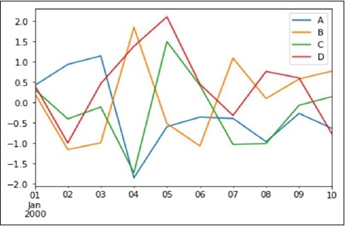
如果索引包含日期,它將呼叫 **gct().autofmt_xdate()** 以格式化 x 軸,如上圖所示。
我們可以使用 **x** 和 **y** 關鍵字繪製一列與另一列的關係圖。
繪圖方法允許使用少數幾種除預設線圖以外的繪圖樣式。這些方法可以作為 **plot()** 的 kind 關鍵字引數提供。這些包括:
- bar 或 barh 用於條形圖
- hist 用於直方圖
- box 用於箱線圖
- 'area' 用於面積圖
- 'scatter' 用於散點圖
條形圖
現在讓我們透過建立一個條形圖來看看什麼是條形圖。條形圖可以透過以下方式建立:
import pandas as pd import numpy as np df = pd.DataFrame(np.random.rand(10,4),columns=['a','b','c','d') df.plot.bar()
其 **輸出** 如下:
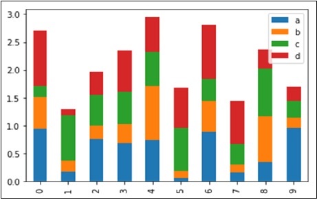
要生成堆疊條形圖,請 **傳遞 stacked=True**:
import pandas as pd df = pd.DataFrame(np.random.rand(10,4),columns=['a','b','c','d') df.plot.bar(stacked=True)
其 **輸出** 如下:
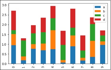
要獲取水平條形圖,請使用 **barh** 方法:
import pandas as pd import numpy as np df = pd.DataFrame(np.random.rand(10,4),columns=['a','b','c','d') df.plot.barh(stacked=True)
其 **輸出** 如下:
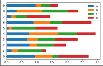
直方圖
可以使用 **plot.hist()** 方法繪製直方圖。我們可以指定箱數。
import pandas as pd
import numpy as np
df = pd.DataFrame({'a':np.random.randn(1000)+1,'b':np.random.randn(1000),'c':
np.random.randn(1000) - 1}, columns=['a', 'b', 'c'])
df.plot.hist(bins=20)
其 **輸出** 如下:
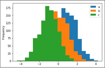
要為每一列繪製不同的直方圖,請使用以下程式碼:
import pandas as pd
import numpy as np
df=pd.DataFrame({'a':np.random.randn(1000)+1,'b':np.random.randn(1000),'c':
np.random.randn(1000) - 1}, columns=['a', 'b', 'c'])
df.diff.hist(bins=20)
其 **輸出** 如下:
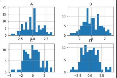
箱線圖
可以透過呼叫 **Series.box.plot()** 和 **DataFrame.box.plot()**,或者 **DataFrame.boxplot()** 來繪製箱線圖,以視覺化每一列中值的分佈。
例如,這是一個箱線圖,它表示在 [0,1) 上進行 10 次觀察的 5 次均勻隨機變數試驗。
import pandas as pd import numpy as np df = pd.DataFrame(np.random.rand(10, 5), columns=['A', 'B', 'C', 'D', 'E']) df.plot.box()
其 **輸出** 如下:
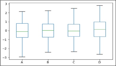
面積圖
可以使用 **Series.plot.area()** 或 **DataFrame.plot.area()** 方法建立面積圖。
import pandas as pd import numpy as np df = pd.DataFrame(np.random.rand(10, 4), columns=['a', 'b', 'c', 'd']) df.plot.area()
其 **輸出** 如下:
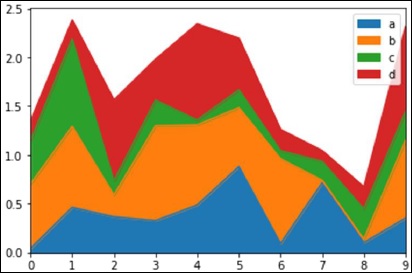
散點圖
可以使用 **DataFrame.plot.scatter()** 方法建立散點圖。
import pandas as pd import numpy as np df = pd.DataFrame(np.random.rand(50, 4), columns=['a', 'b', 'c', 'd']) df.plot.scatter(x='a', y='b')
其 **輸出** 如下:
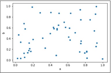
餅圖
可以使用 **DataFrame.plot.pie()** 方法建立餅圖。
import pandas as pd import numpy as np df = pd.DataFrame(3 * np.random.rand(4), index=['a', 'b', 'c', 'd'], columns=['x']) df.plot.pie(subplots=True)
其 **輸出** 如下:
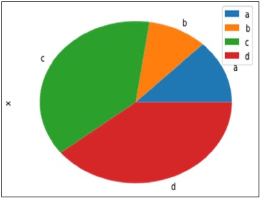
Python Pandas - I/O 工具
**Pandas I/O API** 是一組頂級讀取器函式,類似於 **pd.read_csv()**,通常返回 Pandas 物件。
用於讀取文字檔案(或平面檔案)的兩個主要函式是 **read_csv()** 和 **read_table()**。它們都使用相同的解析程式碼將表格資料智慧地轉換為 **DataFrame** 物件:
pandas.read_csv(filepath_or_buffer, sep=',', delimiter=None, header='infer', names=None, index_col=None, usecols=None
pandas.read_csv(filepath_or_buffer, sep='\t', delimiter=None, header='infer', names=None, index_col=None, usecols=None
以下是 **csv** 檔案資料的樣子:
S.No,Name,Age,City,Salary 1,Tom,28,Toronto,20000 2,Lee,32,HongKong,3000 3,Steven,43,Bay Area,8300 4,Ram,38,Hyderabad,3900
將此資料另存為 **temp.csv** 並對其進行操作。
S.No,Name,Age,City,Salary 1,Tom,28,Toronto,20000 2,Lee,32,HongKong,3000 3,Steven,43,Bay Area,8300 4,Ram,38,Hyderabad,3900
將此資料另存為 **temp.csv** 並對其進行操作。
read.csv
**read.csv** 從 csv 檔案讀取資料並建立 DataFrame 物件。
import pandas as pd
df=pd.read_csv("temp.csv")
print df
其 **輸出** 如下:
S.No Name Age City Salary 0 1 Tom 28 Toronto 20000 1 2 Lee 32 HongKong 3000 2 3 Steven 43 Bay Area 8300 3 4 Ram 38 Hyderabad 3900
自定義索引
這指定了 csv 檔案中的一列,可以使用 **index_col** 來自定義索引。
import pandas as pd
df=pd.read_csv("temp.csv",index_col=['S.No'])
print df
其 **輸出** 如下:
S.No Name Age City Salary 1 Tom 28 Toronto 20000 2 Lee 32 HongKong 3000 3 Steven 43 Bay Area 8300 4 Ram 38 Hyderabad 3900
轉換器
列的 **dtype** 可以作為字典傳遞。
import pandas as pd
df = pd.read_csv("temp.csv", dtype={'Salary': np.float64})
print df.dtypes
其 **輸出** 如下:
S.No int64 Name object Age int64 City object Salary float64 dtype: object
預設情況下,Salary 列的 **dtype** 是 **int**,但結果顯示為 **float**,因為我們已顯式轉換了型別。
因此,資料看起來像浮點數:
S.No Name Age City Salary 0 1 Tom 28 Toronto 20000.0 1 2 Lee 32 HongKong 3000.0 2 3 Steven 43 Bay Area 8300.0 3 4 Ram 38 Hyderabad 3900.0
header_names
使用 names 引數指定 header 的名稱。
import pandas as pd
df=pd.read_csv("temp.csv", names=['a', 'b', 'c','d','e'])
print df
其 **輸出** 如下:
a b c d e 0 S.No Name Age City Salary 1 1 Tom 28 Toronto 20000 2 2 Lee 32 HongKong 3000 3 3 Steven 43 Bay Area 8300 4 4 Ram 38 Hyderabad 3900
觀察到,header 名稱已附加了自定義名稱,但檔案中的 header 尚未刪除。現在,我們使用 header 引數將其刪除。
如果 header 不在第一行,則將行號傳遞給 header。這將跳過前面的行。
import pandas as pd
df=pd.read_csv("temp.csv",names=['a','b','c','d','e'],header=0)
print df
其 **輸出** 如下:
a b c d e 0 S.No Name Age City Salary 1 1 Tom 28 Toronto 20000 2 2 Lee 32 HongKong 3000 3 3 Steven 43 Bay Area 8300 4 4 Ram 38 Hyderabad 3900
skiprows
skiprows 跳過指定數量的行。
import pandas as pd
df=pd.read_csv("temp.csv", skiprows=2)
print df
其 **輸出** 如下:
2 Lee 32 HongKong 3000 0 3 Steven 43 Bay Area 8300 1 4 Ram 38 Hyderabad 3900
Python Pandas - 稀疏資料
當任何與特定值匹配的資料(NaN/缺失值,儘管可以選擇任何值)被省略時,稀疏物件會被“壓縮”。一個特殊的 SparseIndex 物件跟蹤資料被“稀疏化”的位置。在一個例子中,這將更有意義。所有標準的 Pandas 資料結構都應用 **to_sparse** 方法:
import pandas as pd import numpy as np ts = pd.Series(np.random.randn(10)) ts[2:-2] = np.nan sts = ts.to_sparse() print sts
其 **輸出** 如下:
0 -0.810497 1 -1.419954 2 NaN 3 NaN 4 NaN 5 NaN 6 NaN 7 NaN 8 0.439240 9 -1.095910 dtype: float64 BlockIndex Block locations: array([0, 8], dtype=int32) Block lengths: array([2, 2], dtype=int32)
稀疏物件的存在是為了提高記憶體效率。
現在讓我們假設您有一個大型 NA DataFrame 並執行以下程式碼:
import pandas as pd import numpy as np df = pd.DataFrame(np.random.randn(10000, 4)) df.ix[:9998] = np.nan sdf = df.to_sparse() print sdf.density
其 **輸出** 如下:
0.0001
任何稀疏物件都可以透過呼叫 **to_dense** 轉換回標準密集形式:
import pandas as pd import numpy as np ts = pd.Series(np.random.randn(10)) ts[2:-2] = np.nan sts = ts.to_sparse() print sts.to_dense()
其 **輸出** 如下:
0 -0.810497 1 -1.419954 2 NaN 3 NaN 4 NaN 5 NaN 6 NaN 7 NaN 8 0.439240 9 -1.095910 dtype: float64
稀疏 Dtypes
稀疏資料應與其密集表示具有相同的 dtype。目前,支援 **float64、int64** 和 **booldtypes**。根據原始 **dtype,fill_value 預設值** 會發生變化:
**float64** − np.nan
**int64** − 0
**bool** − False
讓我們執行以下程式碼來了解這一點:
import pandas as pd import numpy as np s = pd.Series([1, np.nan, np.nan]) print s s.to_sparse() print s
其 **輸出** 如下:
0 1.0 1 NaN 2 NaN dtype: float64 0 1.0 1 NaN 2 NaN dtype: float64
Python Pandas - 警告和陷阱
Caveats 表示警告,gotcha 表示未發現的問題。
在 Pandas 中使用 If/Truth 語句
Pandas 遵循 numpy 的約定,在嘗試將某些內容轉換為布林值 (bool) 時會引發錯誤。這發生在使用布林運算子 `if` 或 `when`,以及 `and`、`or` 或 `not` 的情況下。結果應該是什麼並不明確。因為它不是零長度,所以應該是 True 嗎?因為存在 False 值,所以應該是 False 嗎?這不明確,因此 Pandas 會引發ValueError。
import pandas as pd if pd.Series([False, True, False]): print 'I am True'
其 **輸出** 如下:
ValueError: The truth value of a Series is ambiguous. Use a.empty, a.bool() a.item(),a.any() or a.all().
在 `if` 條件中,不清楚該如何處理。該錯誤提示是否應該使用 `None` 或其中任何一個。
import pandas as pd
if pd.Series([False, True, False]).any():
print("I am any")
其 **輸出** 如下:
I am any
要在布林上下文中評估單元素 Pandas 物件,請使用 `.bool()` 方法。
import pandas as pd print pd.Series([True]).bool()
其 **輸出** 如下:
True
按位布林運算
像 `==` 和 `!=` 這樣的按位布林運算子將返回一個布林序列,而這幾乎總是需要的。
import pandas as pd s = pd.Series(range(5)) print s==4
其 **輸出** 如下:
0 False 1 False 2 False 3 False 4 True dtype: bool
isin 操作
這將返回一個布林序列,顯示 Series 中的每個元素是否完全包含在傳遞的值序列中。
import pandas as pd
s = pd.Series(list('abc'))
s = s.isin(['a', 'c', 'e'])
print s
其 **輸出** 如下:
0 True 1 False 2 True dtype: bool
重新索引與 ix 的陷阱
許多使用者會發現自己使用ix 索引功能作為從 Pandas 物件中選擇資料的簡潔方法。
import pandas as pd
import numpy as np
df = pd.DataFrame(np.random.randn(6, 4), columns=['one', 'two', 'three',
'four'],index=list('abcdef'))
print df
print df.ix[['b', 'c', 'e']]
其 **輸出** 如下:
one two three four
a -1.582025 1.335773 0.961417 -1.272084
b 1.461512 0.111372 -0.072225 0.553058
c -1.240671 0.762185 1.511936 -0.630920
d -2.380648 -0.029981 0.196489 0.531714
e 1.846746 0.148149 0.275398 -0.244559
f -1.842662 -0.933195 2.303949 0.677641
one two three four
b 1.461512 0.111372 -0.072225 0.553058
c -1.240671 0.762185 1.511936 -0.630920
e 1.846746 0.148149 0.275398 -0.244559
當然,在這種情況下,這與使用reindex方法完全等效。
import pandas as pd
import numpy as np
df = pd.DataFrame(np.random.randn(6, 4), columns=['one', 'two', 'three',
'four'],index=list('abcdef'))
print df
print df.reindex(['b', 'c', 'e'])
其 **輸出** 如下:
one two three four
a 1.639081 1.369838 0.261287 -1.662003
b -0.173359 0.242447 -0.494384 0.346882
c -0.106411 0.623568 0.282401 -0.916361
d -1.078791 -0.612607 -0.897289 -1.146893
e 0.465215 1.552873 -1.841959 0.329404
f 0.966022 -0.190077 1.324247 0.678064
one two three four
b -0.173359 0.242447 -0.494384 0.346882
c -0.106411 0.623568 0.282401 -0.916361
e 0.465215 1.552873 -1.841959 0.329404
根據這一點,有些人可能會得出結論,ix 和reindex是 100% 等效的。除了整數索引的情況外,這是正確的。例如,上述操作可以另一種方式表達為:
import pandas as pd
import numpy as np
df = pd.DataFrame(np.random.randn(6, 4), columns=['one', 'two', 'three',
'four'],index=list('abcdef'))
print df
print df.ix[[1, 2, 4]]
print df.reindex([1, 2, 4])
其 **輸出** 如下:
one two three four
a -1.015695 -0.553847 1.106235 -0.784460
b -0.527398 -0.518198 -0.710546 -0.512036
c -0.842803 -1.050374 0.787146 0.205147
d -1.238016 -0.749554 -0.547470 -0.029045
e -0.056788 1.063999 -0.767220 0.212476
f 1.139714 0.036159 0.201912 0.710119
one two three four
b -0.527398 -0.518198 -0.710546 -0.512036
c -0.842803 -1.050374 0.787146 0.205147
e -0.056788 1.063999 -0.767220 0.212476
one two three four
1 NaN NaN NaN NaN
2 NaN NaN NaN NaN
4 NaN NaN NaN NaN
重要的是要記住,reindex 僅是嚴格的標籤索引。在索引包含整數和字串等病態情況下,這可能會導致一些潛在的意外結果。
Python Pandas - 與 SQL 的比較
由於許多潛在的 Pandas 使用者都熟悉 SQL,因此本頁旨在提供一些關於如何使用 pandas 執行各種 SQL 操作的示例。
import pandas as pd url = 'https://raw.github.com/pandasdev/ pandas/master/pandas/tests/data/tips.csv' tips=pd.read_csv(url) print tips.head()
其 **輸出** 如下:
total_bill tip sex smoker day time size 0 16.99 1.01 Female No Sun Dinner 2 1 10.34 1.66 Male No Sun Dinner 3 2 21.01 3.50 Male No Sun Dinner 3 3 23.68 3.31 Male No Sun Dinner 2 4 24.59 3.61 Female No Sun Dinner 4
SELECT
在 SQL 中,選擇是使用逗號分隔的列列表(或 `*` 選擇所有列)來完成的。
SELECT total_bill, tip, smoker, time FROM tips LIMIT 5;
在 Pandas 中,列選擇是透過將列名列表傳遞給您的 DataFrame 來完成的。
tips[['total_bill', 'tip', 'smoker', 'time']].head(5)
讓我們檢查完整的程式。
import pandas as pd url = 'https://raw.github.com/pandasdev/ pandas/master/pandas/tests/data/tips.csv' tips=pd.read_csv(url) print tips[['total_bill', 'tip', 'smoker', 'time']].head(5)
其 **輸出** 如下:
total_bill tip smoker time 0 16.99 1.01 No Dinner 1 10.34 1.66 No Dinner 2 21.01 3.50 No Dinner 3 23.68 3.31 No Dinner 4 24.59 3.61 No Dinner
在不帶列名列表的情況下呼叫 DataFrame 將顯示所有列(類似於 SQL 的 `*`)。
WHERE
在 SQL 中,過濾是透過 WHERE 子句完成的。
SELECT * FROM tips WHERE time = 'Dinner' LIMIT 5;
DataFrame 可以透過多種方式進行過濾;其中最直觀的是使用布林索引。
tips[tips['time'] == 'Dinner'].head(5)
讓我們檢查完整的程式。
import pandas as pd url = 'https://raw.github.com/pandasdev/ pandas/master/pandas/tests/data/tips.csv' tips=pd.read_csv(url) print tips[tips['time'] == 'Dinner'].head(5)
其 **輸出** 如下:
total_bill tip sex smoker day time size 0 16.99 1.01 Female No Sun Dinner 2 1 10.34 1.66 Male No Sun Dinner 3 2 21.01 3.50 Male No Sun Dinner 3 3 23.68 3.31 Male No Sun Dinner 2 4 24.59 3.61 Female No Sun Dinner 4
上面的語句將一個 True/False 物件的序列傳遞給 DataFrame,返回所有值為 True 的行。
GroupBy
此操作獲取整個資料集中每個組中記錄的數量。例如,查詢獲取按性別留下的消費小費數量:
SELECT sex, count(*) FROM tips GROUP BY sex;
Pandas 等效項將是:
tips.groupby('sex').size()
讓我們檢查完整的程式。
import pandas as pd
url = 'https://raw.github.com/pandasdev/
pandas/master/pandas/tests/data/tips.csv'
tips=pd.read_csv(url)
print tips.groupby('sex').size()
其 **輸出** 如下:
sex Female 87 Male 157 dtype: int64
前 N 行
SQL 使用LIMIT返回前 n 行。
SELECT * FROM tips LIMIT 5 ;
Pandas 等效項將是:
tips.head(5)
讓我們檢查完整的示例。
import pandas as pd url = 'https://raw.github.com/pandas-dev/pandas/master/pandas/tests/data/tips.csv' tips=pd.read_csv(url) tips = tips[['smoker', 'day', 'time']].head(5) print tips
其 **輸出** 如下:
smoker day time 0 No Sun Dinner 1 No Sun Dinner 2 No Sun Dinner 3 No Sun Dinner 4 No Sun Dinner
這些是我們之前章節中學習的 Pandas 庫中比較的幾個基本操作。