MATLAB 中的傅立葉變換卷積定理

---

根據**傅立葉變換的卷積定理**，兩個訊號在時域的卷積等價於它們在頻域的乘積。因此，如果兩個訊號在時域進行卷積，則它們的結果與在頻域對其傅立葉變換進行乘積的結果相同。

例如，如果 x(t) 和 h(t) 是時域中的兩個訊號，它們的傅立葉變換分別為 X(ω) 和 H(ω)。那麼，它們在時域的卷積由下式給出：

f(t) = x(t) * h(t)

這裡，符號“*”表示兩個訊號的卷積。

並且，它們傅立葉變換在頻域的乘積由下式給出：

F(ω) = X(ω).H(ω)

根據卷積定理，函式 f(t) 和 F(ω) 透過傅立葉變換及其逆變換相關聯，如下所示：

F(ω) = fft(x(t) * h(t))

以及

f(t) = ifft(X(ω).H(ω))

這裡，“fft”是 MATLAB 中用於執行輸入訊號傅立葉變換的函式，“ifft”是另一個 MATLAB 函式，用於執行逆傅立葉變換。

總的來說，傅立葉變換的卷積定理允許我們在頻域執行輸入訊號的卷積，這僅僅是一個乘法運算。

現在，讓我們考慮一些 MATLAB 程式，這些程式使用傅立葉變換的卷積定理在時域和頻域執行卷積運算。

示例

% MATLAB program to demonstrate the use of Convolution Theorem of Fourier Transform
% Define two input signals
x = [2 4 6 8];
y = [0.4 0.4 0.4 0.4];
% Calculate the lengths of the input signals
L1 = length(x);
L2 = length(y);
% Calculate the length of the convolution result
L = L1 + L2 - 1;
% Perform zero-padding of the input signals to the length of the convolution result
a = [x zeros(1, L-L1)];
b = [y zeros(1, L-L2)];
% Perform the Fourier Transform of the padded signals a and b
X = fft(a);
Y = fft(b);
% Perform the convolution in the time domain
CT = conv(x, y);
% Perform the convolution in the frequency domain using the Convolution Theorem
CF = ifft(X .* Y);
% Display the results
disp('Convolution of x and y in the time domain is:');
disp(CT);
disp('Convolution of x and y in the frequency domain using the Convolution Theorem is:');
disp(CF);

輸出

Convolution of x and y in the time domain is:
    0.8000    2.4000    4.8000    8.0000    7.2000    5.6000    3.2000

Convolution of x and y in the frequency domain using the Convolution Theorem is:
    0.8000    2.4000    4.8000    8.0000    7.2000    5.6000    3.2000

解釋

在這個 MATLAB 程式中，我們定義了儲存在變數“x”和“y”中的兩個輸入訊號。然後，我們計算輸入訊號的長度和卷積結果的長度，並將它們儲存在變數“L1”、“L2”和“L”中。接下來，我們對訊號“x”和“y”進行零填充，使其長度與卷積結果的長度匹配，並將零填充後的訊號儲存在變數“a”和“b”中。

然後，我們使用“fft”函式獲取零填充訊號“a”和“b”的傅立葉變換。接下來，我們使用“conv”函式在時域執行訊號“x”和“y”的卷積，並將結果儲存在變數“CT”中。

之後，我們在頻域執行“X”和“Y”的乘法，並使用“ifft”函式計算乘積的逆傅立葉變換以獲得卷積結果。

最後，我們使用“disp”函式顯示結果。從輸出中，我們可以觀察到在時域（即“CT”）和使用卷積定理得到的頻域“CF”中獲得的結果是相同的。

示例

% MATLAB program to perform convolution in the spatial domain
% Read the input image
img = imread('https://tutorialspoint.tw/assets/questions/media/14304-1687425236.jpg');
% Convert the image to grayscale if necessary
if size(img, 3) == 3
    img = rgb2gray(img);
end
% Define averaging filter
filter = ones(10) / 50;
% Perform convolution in the spatial domain
C = conv2(double(img), filter, 'same');
% Display the original and filtered images
subplot(1, 2, 1); imshow(img); title('Original Image');
subplot(1, 2, 2); imshow(C, []); title('Convolved Image');

輸出

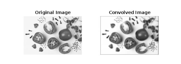
解釋

在這個 MATLAB 程式中，我們使用“imread”函式讀取輸入影像並將其儲存在變數“img”中。接下來，我們檢查輸入影像是灰度影像還是彩色影像。如果不是灰度影像，則使用“rgb2gray”函式將其轉換為灰度影像。然後，我們將平均濾波器定義為一個 10 × 10 的矩陣，所有元素都設定為 1/50，它表示一個簡單的盒式濾波器。

之後，我們使用“conv2”函式在空間域執行影像的卷積。在這裡，我們還使用“double()”函式將影像轉換為雙精度以執行浮點計算。

最後，我們使用“imshow”函式顯示原始影像和卷積後的影像。這裡，“[]”用於自動縮放卷積影像的值。

示例

% MATLAB program to perform convolution in frequency domain
% Read the input image
I = imread('https://tutorialspoint.tw/assets/questions/media/14304-1687425236.jpg');
% Convert the colored image to grayscale if necessary
if size(I, 3) == 3
    I = rgb2gray(I);
end
% Define averaging filter
filter = ones(10) / 50;
% Calculate the Fourier Transform of the image and the filter
Img_FT = fftshift(fft2(I));
Flt_FT= fftshift(fft2(filter, size(I, 1), size(I, 2)));
% Perform convolution in the frequency domain
C = ifft2(ifftshift(Img_FT .* Flt_FT));
% Display the Fourier Transforms of the image, filter, original image, and convolved image
FT_Image = abs(log(Img_FT));
FT_Filter = abs(log(Flt_FT));
subplot(1, 4, 1), imshow(FT_Image, []); title('FT Image');
subplot(1, 4, 2), imshow(FT_Filter, []); title('FT Filter');
subplot(1, 4, 3), imshow(I, []); title('Original Image');
subplot(1, 4, 4), imshow(C, []); title('Convolved Image');

輸出

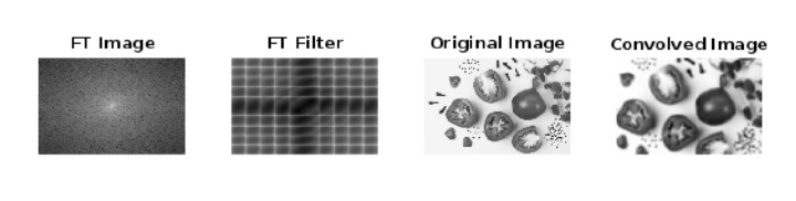
解釋

在這個 MATLAB 程式碼中，我們首先使用“imread”函式讀取輸入影像並將輸入影像儲存在“I”變數中。然後，如果需要，我們將影像轉換為灰度影像，為此我們使用“rgb2gray”函式。

接下來，我們將平均濾波器“filter”定義為一個 10 × 10 的矩陣，所有元素都設定為 1/50，它是一個簡單的盒式濾波器。

之後，我們使用“fft2”函式計算輸入影像和濾波器的傅立葉變換。在這裡，我們還使用“fftshift”函式將零頻率分量移到中心，以便更好地視覺化。

接下來，我們在頻域執行傅立葉變換後的影像“Img_FT”和傅立葉變換後的濾波器“Flt_FT”的乘法。此外，我們計算逆傅立葉變換以獲得卷積後的影像，為此我們使用“ifft2”和“ifftshift”函式。

最後，我們使用“imshow”函式顯示傅立葉變換後的影像、傅立葉變換後的濾波器、原始影像和卷積後的影像。這裡，“[]”用於自動縮放影像的值。

因此，這就是關於 MATLAB 中傅立葉變換卷積定理的所有內容。