
 資料結構
資料結構 網路
網路 關係資料庫管理系統 (RDBMS)
 作業系統
作業系統 Java
Java iOS
iOS HTML
HTML CSS
CSS Android
 Python
 C語言程式設計
 C++
C++ C#
C# MongoDB
 MySQL
MySQL Javascript
 PHP
PHP利用拉普拉斯變換進行電路分析
拉普拉斯變換
拉普拉斯變換是一種數學工具,用於將時域中的微分方程轉換為頻域或s域中的代數方程。
數學上,如果$\mathrm{\mathit{x\left(t\right)}}$是時域函式,則其拉普拉斯變換定義為:
$$\mathrm{\mathit{L\left[\mathit{x}\mathrm{\left(\mathit{t} \right )}\right ]\mathrm{=}X\mathrm{\left ( \mathit{s}\right)}\mathrm{=}\int_{-\infty }^{\infty}x\mathrm{\left (\mathit{t} \right )}e^{-st} \:dt}}$$
利用拉普拉斯變換進行電路分析
拉普拉斯變換可以用來解決不同的電路問題。為了解決電路問題,首先需要寫出電路的微分方程,然後利用拉普拉斯變換求解這些微分方程。此外,電路本身也可以使用拉普拉斯變換轉換為s域,然後寫出並求解對應的電路代數方程。
電路可以包含三種電路元件:電阻器(R)、電感器(L)和電容器(C),下面將討論使用拉普拉斯變換分析這些元件的方法。
純電阻電路
圖1顯示了一個由純電阻元件組成的電路。
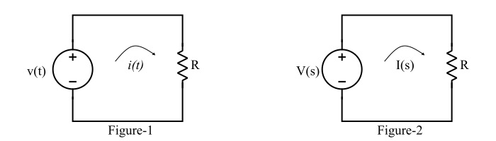
透過在這個電路中應用基爾霍夫電壓定律(KVL),我們可以寫出:
$$\mathrm{\mathit{v\mathrm{\left(\mathit{t}\right )}\mathrm{=}Ri\mathrm{\left ( \mathit{t}\right)}}}$$
因此,該方程的拉普拉斯變換為:
$$\mathrm{\mathit{V\mathrm{\left(\mathit{s}\right )}\mathrm{=}RI\mathrm{\left ( \mathit{s}\right)}}}$$
這裡需要注意的是,時域中的電阻R在s域中仍然是R。該電路的拉普拉斯變換版本如圖2所示。
純電感電路
圖3顯示了一個由純電感器組成的電路。
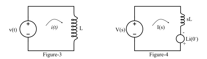
純電感元件的電壓方程為:
$$\mathrm{\mathit{v\mathrm{\left(\mathit{t}\right)}\mathrm{=} L\frac{di\mathrm{\left(\mathit{t} \right )}}{dt}}}$$
對等式兩邊進行拉普拉斯變換,得到:
$$\mathrm{\mathit{V\mathrm{\left(\mathit{s}\right)}\mathrm{=} \mathrm{\left[\mathit{sI}\mathrm{\left (\mathit{s} \right)}-\mathit{i\mathrm{\left (0^{-} \right )}}\right]}L}}$$
$$\mathrm{\Rightarrow \mathit{V\mathrm{\left(\mathit{s}\right)}\mathrm{=} sLI\mathrm{\left ( \mathit{s}\right)-\mathit{Li}\mathrm{\left ( 0^{-}\right )}}}}$$
其中,$i\mathrm{\left ( 0^{-}\right )}$是流過電感的初始電流。
時域中元件的電感($\mathit{L}$)在s域中變為sL。此外,電路電流$I\mathrm{\left(\mathit{s}\right)}$受到電壓$Li\mathrm{\left(\mathrm{0^{-}}\right)}$的阻礙。純電感電路的拉普拉斯變換版本如圖4所示。
純電容電路
圖5顯示了一個由純電容元件組成的電路。
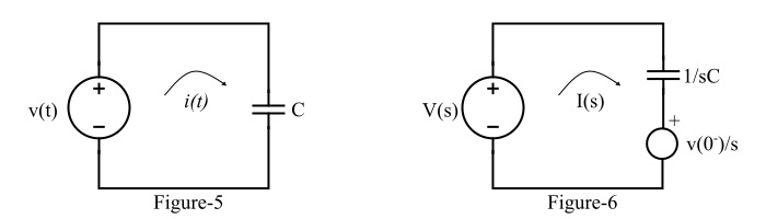
流過電容器的電流為:
$$\mathrm{\mathit{i}\mathrm{\left(\mathit{t}\right)}\mathrm{=}\mathit{C\:\frac{dv\left(t\right )}{dt}}}$$
對該方程進行拉普拉斯變換,得到:
$$\mathrm{\mathit{I}\mathrm{\left(\mathit{s}\right)}\:\mathrm{=}\:\mathit{C}\mathrm{\left[ \mathit{sV\mathrm{\left(s\right)-\mathit{v}\mathrm{\left ( 0^{-} \right )}}}\right ]}\mathrm{=}sCV\mathrm{\left ( s \right )-\mathit{Cv}\mathrm{\left ( 0^{-} \right )}}}$$
$$\mathrm{\therefore \mathit{I}\mathrm{\left(\mathit{s}\right)}\:\mathrm{=}\:sCV\mathrm{\left ( \mathit{s} \right )-\mathit{q}\mathrm{\left ( 0^{-} \right )}}}$$
同時
$$\mathrm{\mathit{V\mathrm{\left ( \mathit{s} \right )}\mathrm{=}\frac{\mathrm{1}}{\mathit{sC}}I\mathrm{\mathit{\left (s\right )}}}+\frac{\mathrm{1}}{\mathit{sC}}\mathit{q}\mathrm{\mathit{\left (\mathrm{0^{-}}\right )}}}$$
$$\mathrm{\therefore \mathit{V\mathrm{\left ( \mathit{s} \right )}\mathrm{=}\frac{I\mathrm{\left (\mathit{s} \right)}}{sC}\mathrm{+}\frac{v\mathrm{\left(\mathrm{0^{-}} \right )}}{s}}}$$
其中,$\mathrm{\mathit{v\mathrm{\left ( 0^{-} \right )}}}$是電容器兩端的初始電壓。
很明顯,時域中的電容(C)在s域中變為$\mathrm{\left(\frac{1}{\mathit{sc}}\right )}$。此外,在s域中引入了電壓$\mathrm{\left [\frac{\mathit{v}\mathrm{\left ( 0^{-} \right )}}{\mathit{s}} \right ]}$,它阻礙了電路電流的流動。純電容電路的拉普拉斯變換版本如圖6所示。

19K+ 瀏覽量
