使用 Python 展示統計學中的 Pearson III 型分佈

---

Pearson III 型分佈是一種在統計學中廣泛使用的連續機率分佈。它具有偏斜分佈。三個引數決定了分佈的形狀：位置、尺度和形狀。發現這種型別的分佈將使統計學家能夠更有效地分析資料並做出更精確的預測。

我們可以使用 `pearson3.rvs` 函式從分佈中生成隨機數，並藉助 `pearson3.pdf` 函式計算給定點的機率密度函式 (pdf)。

Pearson III 型分佈的引數

• 形狀引數 - 此引數透過分佈的機率密度確定分佈的擴充套件程度。最大值應為 0。當此值小於 0 時，分佈是擴充套件的。

• 位置引數 - 此引數決定分佈圖的位置。它應該為零。

• 尺度引數 - 此引數決定分佈圖的尺度。最大值應為 0。當此值小於 0 時，分佈是擴充套件的。

語法

用於從分佈中生成隨機數。

ran_num = pearson3.rvs(shape, loc, scale, size)

方法 1：這裡我們正在計算來自給定分佈的隨機數

示例 1

從分佈中生成 12 個隨機數。

from scipy.stats import pearson3

#parameters of the Pearson Type 3 distribution
shape = 2.7
loc = 1.0
scale = 0.7

# Generating random numbers from the distribution
ran_num = pearson3.rvs(shape, loc, scale, size=12)
# Print the numbers
print(ran_num)

輸出

[1.78675698 1.2868774  0.79792263 1.73894349 1.06018355 0.90932737
 1.03330347 0.79210384 0.61598714 0.5778327  0.4899408  0.72123621]

在這個例子中，我們首先定義了三個引數（形狀、位置、尺度），然後應用 `pearson3.rvs` 函式生成 12 個隨機數。

示例 2

從分佈中生成並繪製 12 個隨機數的直方圖。

from scipy.stats import pearson3
import matplotlib.pyplot as plt

#parameters of the Pearson Type 3 distribution
shape = 2.7
loc = 1.0
scale = 0.7

# Generating random numbers from the distribution
ran_num = pearson3.rvs(shape, loc, scale, size=12)

# histogram of the generated random numbers
plt.hist(ran_num, bins=15)  #bins define the number of bars 
plt.xlabel('Random Numbers')
plt.ylabel('Frequency')
plt.title('Histogram of Random Numbers')
plt.show()

輸出

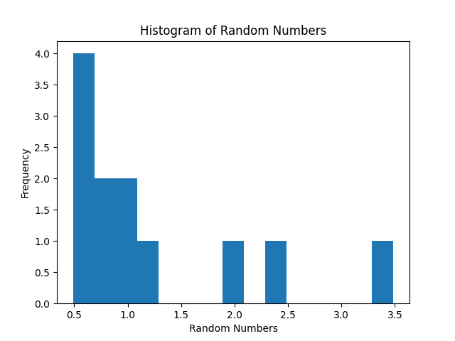
在這個例子中，我們首先定義了三個引數（形狀、位置、尺度），然後應用 `pearson3.rvs` 函式生成 12 個隨機數。最後，我們繪製了直方圖來測量這些隨機數。

示例 3

計算從分佈中生成的 12 個隨機數的均值和中位數。

from scipy.stats import pearson3
import numpy as np

#parameters of the Pearson Type 3 distribution
shape = 2.7
loc = 1.0
scale = 0.7

# Generating random numbers from the distribution
ran_num = pearson3.rvs(shape, loc, scale, size=12)

# Calculating the mean and median of the generated random numbers
mean = np.mean(ran_num)
median = np.median(ran_num)

print("Mean:", mean)
print("Median:", median)

輸出

Mean: 0.7719624059755859
Median: 0.6772205996213376

在這個例子中，我們首先定義了三個引數（形狀、位置、尺度），然後應用 `pearson3.rvs` 函式生成 12 個隨機數，之後我們計算這 12 個隨機數的均值和中位數。

方法 2：這裡我們正在計算來自給定分佈的機率密度函式

語法

用於計算來自分佈的機率密度函式。

pdf = pearson3.pdf(value, shape, loc, scale)

示例 1

計算特定點上分佈的機率密度函式 (pdf)。

import numpy as np
import matplotlib.pyplot as plt
from scipy.stats import pearson3

# parameters of the Pearson Type III distribution
shape = 2.7
loc = 1.0
scale = 0.7

# Calculate the PDF of the distribution on specific point
value = 3.5
pdf = pearson3.pdf(value, shape, loc, scale)

print(pdf)

輸出

0.015858643122817345

在這個例子中，我們定義了三個引數並給定一個特定值。然後應用 `pearson3.pdf` 函式計算機率密度函式。

示例 2

計算範圍為 0 到 10 的分佈的機率密度函式 (pdf)。

import numpy as np
import matplotlib.pyplot as plt
from scipy.stats import pearson3

# parameters of the Pearson Type III distribution
shape = 2.7
loc = 1.0
scale = 0.7


# range of values
value = np.linspace(0, 10, 50)

# Calculate the PDF of the distribution
pdf = pearson3.pdf(value, shape, loc, scale)

print(pdf)

輸出

[0.00000000e+00 0.00000000e+00 0.00000000e+00 1.38886232e+00
 7.32109657e-01 4.75891782e-01 3.31724610e-01 2.39563951e-01
 1.76760034e-01 1.32313927e-01 1.00074326e-01 7.62827095e-02
 5.85022291e-02 4.50857115e-02 3.48854378e-02 2.70832764e-02
 2.10857325e-02 1.64563072e-02 1.28704163e-02 1.00845296e-02
 7.91457807e-03 6.22057784e-03 4.89551703e-03 3.85722655e-03
 3.04237200e-03 2.40197479e-03 1.89804851e-03 1.50105698e-03
 1.18798272e-03 9.40852230e-04 7.45605438e-04 5.91225860e-04
 4.69069138e-04 3.72343273e-04 2.95705253e-04 2.34947290e-04
 1.86752271e-04 1.48502788e-04 1.18131774e-04 9.40054875e-05
 7.48317202e-05 5.95877020e-05 4.74634014e-05 3.78168933e-05
 3.01391876e-05 2.40264885e-05 1.91582965e-05 1.52801078e-05
 1.21897366e-05 9.72649439e-06]

在這個例子中，我們定義了三個引數並給定範圍為 0 到 10 的值。然後應用 `pearson3.pdf` 函式計算機率密度函式並列印結果。

示例 3

分佈的機率密度函式 (pdf) 的視覺化表示。

import numpy as np
import matplotlib.pyplot as plt
from scipy.stats import pearson3

# parameters of the Pearson Type III distribution
shape = 2.7
loc = 1.0
scale = 0.7

# range of values
value = np.linspace(0, 10, 50)

# Calculate the PDF of the distribution
pdf = pearson3.pdf(value, shape, loc, scale)

# Plotting the PDF
plt.plot(value, pdf)
plt.xlabel('value')
plt.ylabel('PDF')
plt.title('Probability Density Function (PDF)')
plt.show()

輸出

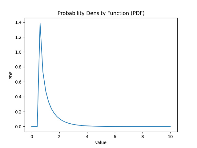
在這個例子中，我們可以看到機率密度函式的圖形表示。

結論

總之，Pearson III 型分佈是一個重要的機率分佈。這種分析在機率論和統計學中佔有重要地位。我們可以使用各種庫和包，例如 SciPy、NumPy 和 Pandas，在 Python 中對 Pearson III 型分佈進行建模。