使用 Python 展示統計學中的非中心卡方分佈

---

在給定的問題陳述中，我們需要藉助 Python 展示非中心卡方分佈。因此，我們將使用 Python 庫來展示所需的結果。

理解非中心卡方分佈

非中心卡方分佈是統計學中的一種機率分佈。這種分佈主要用於功效分析。它是卡方分佈的推廣。它可以透過對標準正態隨機變數的平方求和得到。其中，分佈的形狀由自由度定義。它包含一個非中心引數。此引數表示在分析資料時存在非零效應或訊號。

非中心卡方分佈主要有兩個引數。第一個引數是稱為“df”的自由度，非中心引數稱為“nc”。這裡的自由度表示分佈的形狀，非中心引數表示分佈的位置或偏移。因此，透過更新或操作這兩個值，我們可以建立各種場景。

非中心卡方分佈也可以用於訊號處理和無線通訊等應用。

上述問題的邏輯

為了在 Python 中展示非中心卡方分佈，我們將使用 scipy.stats.ncx2() 函式，該函式表示 Python 中的非中心卡方連續隨機變數。它繼承了 rv_continous 類的通用方法。它還允許我們對與該分佈相關的詳細分析和計算。

演算法

• 步驟 1 - 首先匯入 Python 的必要庫以顯示非中心卡方分佈。在我們的程式中，我們正在匯入 Numpy、Matplotlib 和 Scipy.stats 庫。

# Import the necessary libraries
import numpy as nmp
import matplotlib.pyplot as mt_plt
from scipy.stats import ncx2

• 步驟 2 - 匯入庫後，我們將初始化非中心卡方分佈的引數，例如自由度 df 和非中心引數 nc。

# Initiate the parameters of the distribution
df = 5
nc = 2

• 步驟 3 - 現在，我們將建立一個名為 dist 的非中心卡方分佈物件。它的值將使用 ncx2() 函式計算，並將上述兩個引數傳遞給此函式。並生成用於繪製分佈的 x 座標值。

# Initiate a distribution object
dist = ncx2(df, nc)

# Generate x-values for plotting the distribution
x = nmp.linspace(0, 20, 100)

• 步驟 4 - 接下來，我們將使用 dist() 函式計算機率密度函式 (pdf) 和累積分佈函式 (cdf) 的值。

# Calculate the values of PDF and CDF
pdf = dist.pdf(x)
cdf = dist.cdf(x)

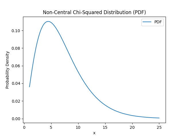
• 步驟 5 - 計算所有所需的值後，我們將使用 matplotlib 繪製機率密度函式。

# Plotting the Probability Density Function
mt_plt.figure()
mt_plt.title('Non-Central Chi-Squared Distribution (PDF)')
mt_plt.plot(x, pdf, label='PDF')
mt_plt.xlabel('x')
mt_plt.ylabel('Probability Density')
mt_plt.legend()

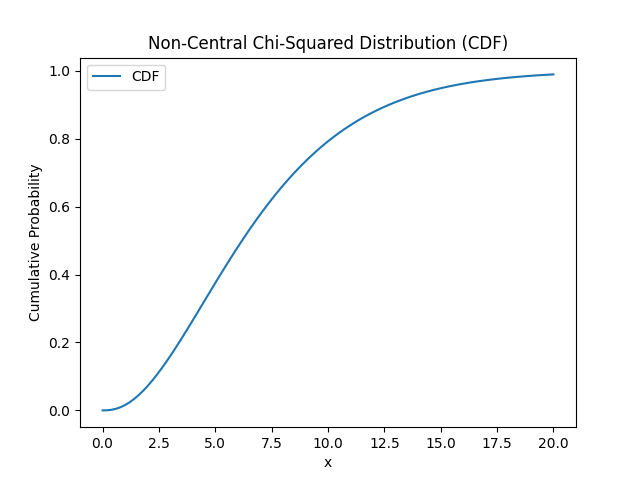
• 步驟 6 - 現在，我們還將使用 matplotlib 庫繪製累積分佈函式。

# Plot the Cumulative Density Function
mt_plt.figure()
mt_plt.title('Non-Central Chi-Squared Distribution (CDF)')
mt_plt.plot(x, cdf, label='CDF')
mt_plt.xlabel('x')
mt_plt.ylabel('Cumulative Probability')
mt_plt.legend()

• 步驟 7 - 最後，我們將使用 show() 函式顯示繪圖。

# Show the distribution
mt_plt.show()

示例

# Import the necessary libraries
import numpy as nmp
import matplotlib.pyplot as mt_plt
from scipy.stats import ncx2

# Initiate the parameters of the distribution
df = 5
nc = 2

# Initiate a distribution object
dist = ncx2(df, nc)

# Generate x-values for plotting the distribution
x = nmp.linspace(0, 20, 100)

# Calculate the values of PDF and CDF
pdf = dist.pdf(x)
cdf = dist.cdf(x)

# Plotting the Probability Density Function
mt_plt.figure()
mt_plt.title('Non-Central Chi-Squared Distribution (PDF)')
mt_plt.plot(x, pdf, label='PDF')
mt_plt.xlabel('x')
mt_plt.ylabel('Probability Density')
mt_plt.legend()

# Plot the Cumulative Density Function
mt_plt.figure()
mt_plt.title('Non-Central Chi-Squared Distribution (CDF)')
mt_plt.plot(x, cdf, label='CDF')
mt_plt.xlabel('x')
mt_plt.ylabel('Cumulative Probability')
mt_plt.legend()

# Show the distribution
mt_plt.show()

輸出

$$\mathrm{非中心卡方分佈 (CDF)}$$

複雜度

顯示非中心卡方分佈的時間複雜度為 O(n)，其中 n 是 x 值的數量。在我們的程式碼中，x 值的範圍是 100。由於我們使用了 plot() 方法來繪製 pdf 和 cdf，這需要 O(n) 時間才能完成任務。

結論

我們已成功使用 Python 的 numpy、matplotlib 和 scipy 庫生成了非中心卡方分佈。我們展示了機率密度函式 (pdf) 和累積分佈函式 (cdf) 的分佈。非中心卡方分佈是一種統計分佈，它使用非中心引數來顯示偏差。因此，透過操作引數，我們可以建立各種場景來建立分佈。