用Python建模朗肯迴圈

---

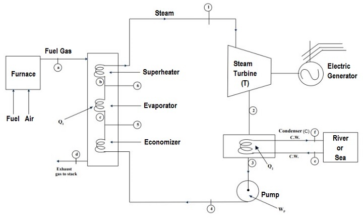
朗肯迴圈是任何熱電廠的核心。基本的朗肯迴圈有四個過程，即汽輪機和泵中的可逆絕熱功相互作用，以及鍋爐和冷凝器中的等壓熱相互作用。

熱電廠示意圖如下所示。

為了提高朗肯迴圈的效率，使用了再生，即將蒸汽從汽輪機中抽出，並將其與給水混合在給水加熱器中。迴圈中的不同過程必須藉助蒸汽表中的資料進行建模。因此，在程式碼本身中擁有資料就變得非常重要。

值得慶幸的是，Pyromat模組可以提供飽和狀態和過熱狀態下的蒸汽資料。讓我們透過一個例子來演示Pyromat的使用及其建模迴圈的能力。

示例1

考慮使用蒸汽作為工作流體的再生迴圈。蒸汽離開鍋爐，以4 MPa，400 °C的壓力進入汽輪機。膨脹到400 kPa後，一些蒸汽從汽輪機中抽出，以在開式FWH中加熱給水。FWH中的壓力為400 kPa，離開FWH的水為400 kPa下的飽和液體。未抽出的蒸汽膨脹到10 kPa。確定迴圈效率。

解決方案

該過程可以示意性地表示為：

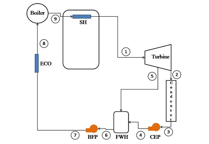
這裡：

• SH - 過熱器

• CEP - 冷凝水抽出泵

• FWH - 給水加熱器

• BFP - 鍋爐給水泵

• ECO - 節能器

• SH - 過熱器

用於模擬朗肯迴圈的Python程式

用於模擬它的Python程式如下：

示例

# Importing the pyromat module
from pyromat import*

# configuring the pressure and fluid
config["unit_pressure"]="kPa"
prop_water=get('mp.H2O')

# Input data
# Boiler exit pressure and temperature
p1=4000
T1=400+273

# Economiser exit pressure
p8=p1

# Economiser inlet pressure
p7=p1

# Steam extraction pressure
p5=400

# Inlet pressure from BFP
p6=p5

# Exit pressure from CEP
p4=p5

# Condenser pressure
p2=10
p3=p2

# Boiler exit pressure
p9=p8

# Turbine
# POINT-1
h1=prop_water.h(p=p1,T=T1)
s1=prop_water.s(p=p1,T=T1)
s5=s1
s2=s1

# POINT-5
T5,x5=prop_water.T_s(p=p5,s=s5,quality='True')
h5=prop_water.h(p=p5,x=x5)

# POINT-2
T2,x2=prop_water.T_s(p=p2,s=s2,quality='True')
h2=prop_water.h(p=p2,x=x2)

# Condenser
# POINT-3
h3=prop_water.hs(p=p3)[0]
T3=prop_water.Ts(p=p3)
s3=prop_water.ss(p=p3)[0]

# CEP
v3=1/prop_water.ds(p=p3)[0]
w_cep=v3*(p4-p3)

# POINT-4
s4=s3
h4=h3+w_cep
T4=prop_water.T_s(s=s4,p=p4)

# FWH
# POINT-6
h6=prop_water.hs(p=p6)[0]
s6=prop_water.ss(p=p6)[0]
T6=prop_water.Ts(p=p6)
v6=1/prop_water.ds(p=p6)[0]

# BFP
# POINT-7
s7=s6
w_bfp=v6*(p7-p6)
h7=h6+w_bfp
T7=prop_water.T_s(s=s7,p=p7)

# POINT-8
h8=prop_water.hs(p=p8)[0]
s8=prop_water.ss(p=p8)[0]
T8=prop_water.Ts(p=p8)

# POINT-9
s9=prop_water.ss(p=p8)[1]
T9=T8

# Final Calculations

# Calculation of extracted mass
m=(h6-h4)/(h5-h4)
w_turbine=h1-h5+(1-m)*(h5-h2)
w_net=w_turbine-w_cep-w_bfp
q1=h1-h7
q2=(1-m)*(h2-h3)

# Method 1
efficiency=(w_net/q1)*100

# Method 2
e2=(1-q2/q1)*100

print('The efficiency of Rankine Cycle is: ',round(e2[0],2),'%')
print('The efficiency of Rankine Cycle is: ',round(efficiency[0],2),'%')

輸出

執行此程式時，將產生以下輸出：

The efficiency of Rankine Cycle is: 37.46 %
The efficiency of Rankine Cycle is: 37.45 %

為了瞭解不同點的溫度和壓力，可以編寫以下程式碼：

from pandas import *
p=[p1,p2,p3,p4,p5,p6,p7,p8,p9]
T=[T1,T2,T3,T4,T5,T6,T7,T8,T9]
stage=list(range(1,10))
data={'stage':stage,'p':p,'T':T}
df=DataFrame(data)
print(df)

輸出將是：

    stage      p                     T
0       1   4000                   673
1       2     10  [318.95560780290276]
2       3     10  [318.95560780290276]
3       4    400    [318.968869853315]
4       5    400   [416.7588812509273]
5       6    400   [416.7588812509273]
6       7   4000   [417.1315355843229]
7       8   4000   [523.5036113863505]
8       9   4000   [523.5036113863505]

要繪製朗肯迴圈，可以使用以下程式碼：

# Importing modules
from pylab import *
from numpy import *

# Setting fonts
font = {'family':'Times New Roman', 'size': 14}
figure(figsize=(7.20, 5.20))
title('Rankine Cycle with Feed water heating (T-s Diagram)',color='b')
rc('font', **font)

# Drawing vapour dome

p=linspace(1,22064,1000)
T=prop_water.Ts(p=p)
s=prop_water.ss(p=p)
plot(s[0],T,'b--',linewidth=2)
plot(s[1],T,'r--',linewidth=2)

# connecting all states with lines
se=[s1,s5,s2,s3,s4,s6,s7,s8,s9,s1]
Te=[T1,T5,T2,T3,T4,T6,T7,T8,T9,T1]
plot(se,Te,'k',linewidth=3)
plot([s5,s6],[T5,T6],'r',linewidth=3)
xlim(0,9)

# Numbering the states
text(s1+0.1,T1,'1')
text(s5+0.1,T5,'5')
text(s2+0.3,T2,'2')
text(s3-0.3,T3,'3')
text(s4-0.3,T4+15,'4')
text(s6-0.3,T6,'6')
text(s7-0.3,T7+15,'7')
text(s8-0.3,T8,'8')
text(s9+0.1,T9-4,'9')
text((s5+s6)/2,(T5)+10,'m')
text((s3+s2)/2+0.3,(T3)+10,'1-m')
xlabel('Entropy (kJ/kg-K)')
ylabel('Temperature (K)')
savefig("Rankine.jpg")
show()

因此，上述程式碼生成的朗肯迴圈圖如下：

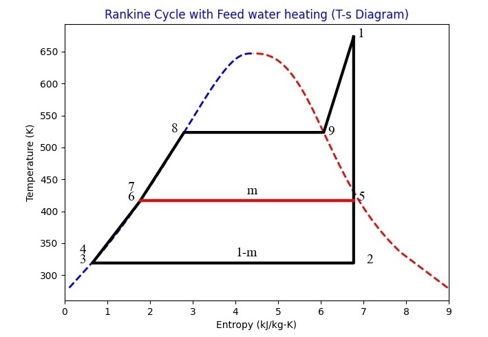
結論

在本簡短教程中，使用Pyromat模組在Python中對朗肯迴圈進行了建模。在使用Pyromat之前，您應該安裝它（對於pip使用者：“pip install pyromat”）。評估並列印不同點的屬性。基於屬性資料，最終繪製了朗肯迴圈。