
 資料結構
資料結構 網路
網路 RDBMS
RDBMS 作業系統
作業系統 Java
Java iOS
iOS HTML
HTML CSS
CSS Android
 Python
 C 程式設計
 C++
C++ C#
C# MongoDB
 MySQL
MySQL Javascript
 PHP
PHP使用 Python 建模牛頓-拉夫森方法
在本教程中,我將向您展示如何藉助稱為牛頓-拉夫森方法的數值方法來評估多項式或超越方程的根。這是一種迭代方法,我們從一個初始猜測(自變數)開始,然後根據猜測評估 𝑥 的新值。並且該過程持續進行,直到達到收斂。該方法透過下圖所示的圖表進行解釋。
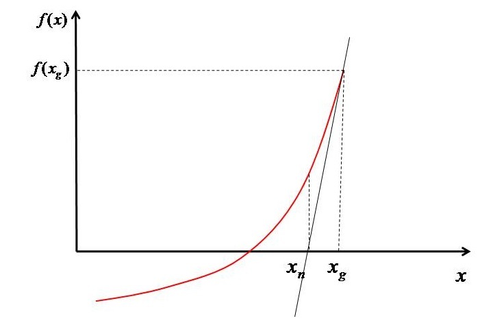
基於 $x_{g}$,評估函式 $(f^{'} \left ( x_{g} \right ))$ 的值。然後在該點繪製一條切線,使其與 𝑥 軸相交於 $x_{n}$。現在我們有兩個點 $(x_{g},f\left ( x_{g} \right ))$ 和 $(x_{n} ,0)$。透過這些點經過的直線的斜率可以寫成公式 1 所示。
$$\mathrm{f^{'} \left ( x_{g} \right )=\frac{0-f\left ( x_{g} \right )}{x_{n}-x_{g}}}$$
因此,$x_{n}$ 可以計算為 -
$$\mathrm{x_{n}-x_{_{g}}=-\frac{f\left ( x_{g} \right )}{f^{'}\left ( x_{g} \right )}}$$
$$\mathrm{x_{n}=x_{_{g}}-\frac{f\left ( x_{g} \right )}{f^{'}\left ( x_{g} \right )}}$$
現在,這個新的 x 值將作為下一步的猜測。基於這個新的猜測,再次評估函式的值,再次評估斜率,並重復該過程,直到獲得根 $(i.e\left | x_{g} -x_{n}\right |<10^{-5})$。
該方法速度很快,但一次只能給你一個根。要獲得另一個根,您必須從另一個猜測開始並再次重複該過程。
牛頓-拉夫森方法的 Python 實現
假設我們想找到方程 $x^{2}+4x+3=0$ 的根。牛頓-拉夫森方法的 Python 實現如下 -
匯入包 -
from pylab import *
只使用了一個模組,即 pylab,因為它包含 numpy。因此,無需單獨匯入它。
形成多項式及其導數函式,即 𝑓(𝑥) 和 𝑓'(x)。
f=lambda x: x**2+4*x+3
dfdx=lambda x: 2*x+4
我使用了 'lambda',因為函式中只有一條語句。如果需要,也可以使用 'def' 方法。
使用 "linspace" 函式為 "x" 建立一個數組。
# Array of x
x=linspace(-15,10,50)
現在,此步驟是可選的。考慮適當的域繪製函式。我還將向您展示如何繪製切線,以及解決方案如何收斂。因此,如果您對視覺效果感興趣,則可以遵循此步驟。
# Plotting the function
figure(1,dpi=150)
plot(x,f(x))
plot([-15,10],[0,0],'k--')
xlabel('x')
ylabel('f(x)')
假設 𝑥 的初始猜測以開始第一次迭代。還將誤差 $(\left | x_{g}-x_{n} \right |)$ 設定為大於收斂標準的值。在本文中,我將收斂標準設定為 $<10^{-5}$,但您可以根據所需的精度級別進行設定。並將迴圈計數器設定為 1。
# Initial Guess
xg=10

# Setting initial error and loop counter
error=1
count=1
在 "for" 迴圈中,使用上述收斂標準求解公式 (2)。此外,繪製誤差和切線。切線繪製在名為 figure(1) 的繪圖中,誤差在 figure(2) 中。此外,還將 $x_{g}$ 和 $f\left ( x_{g} \right )$ 製成表格以顯示不同的值。
# For printing x_g and f(x_g) at different steps
print(f"{'xg':^15}{'f(xg)':^15}")
print("===========================")

# Starting iterations
while error>1.E-5:
   # Solving Eq. 1
   xn=xg-f(xg)/dfdx(xg)

   # Printing x_g and f(x_g)
   print(f'{round(xg,5):^15}{round(f(xg),5):^15}')

   # Plotting tangents
   figure(1,dpi=300)
   plot([xg,xn],[f(xg),0])
   plot([xn,xn],[0,f(xn)],'--',label=f'xg={xg}')
   legend(bbox_to_anchor=(1.01, 1),loc='upper left', borderaxespad=0)

   # Evaluating error and plotting it
   error=abs(xn-xg)
   figure(2,dpi=300)
   semilogy(count,error,'ko')
   xlabel('Iteration count')
   ylabel('Error')

   # Setting up new value as guess for next step
   xg=xn

   # Incrementing the loop counter
   count=count+1
# printing the final answer
print("===========================")
print("\nRoot ",round(xn,5))
show()
收斂後,列印根。並顯示繪圖。
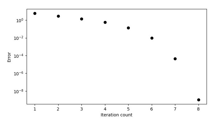
在上述情況下,我將初始猜測設為 10。因此,程式輸出將如下所示 -
      xg                    f(xg)
======================================
      10                     143
    4.04167             35.50174
    1.10359              8.63228
    -0.2871               1.93403
   -0.85165              0.31871
   -0.99042              0.01926
   -0.99995               9e-05
     -1.0                    0.0
========================================
Root -1.0
誤差圖如下所示 -
帶有切線的函式圖在下圖中顯示。
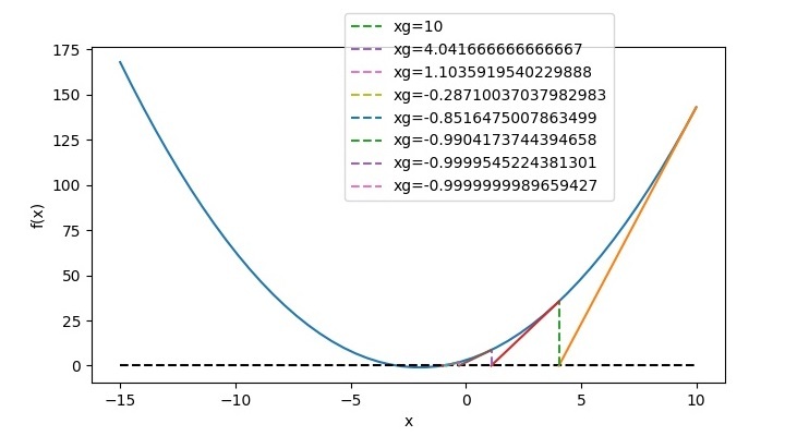
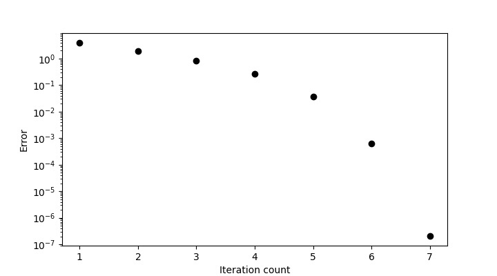
因此,對應於 $x_{g}=10$,根為 -1。對於第二個根,我們必須更改猜測,將其設為 -10。然後程式輸出將如下所示 -
      xg          f(xg)
===========================
       -10          63
     -6.0625     15.50391
    -4.15433      3.64112
    -3.30925      0.71415
    -3.03652      0.07438
    -3.00064      0.00129
    -3.0            0.0
===========================
Root -3.0
現在,誤差圖將如下所示 -
函式圖將如下所示 -
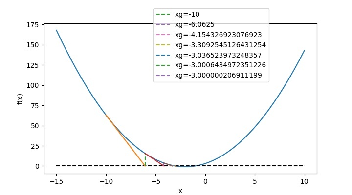
因此,對應於 $x_{g}=-10$,根為 -3。
完整 Python 程式碼
完整程式碼如下 -
# Importing module
from pylab import *

# Funciton for f(x) and f'(x)
f = lambda x: x ** 2 + 4 * x + 3
dfdx = lambda x: 2 * x + 4

# Array of x
x = linspace(-15, 10, 50)

# Plotting the function
figure(1, figsize=(7.20, 4.00))
plot(x, f(x))
plot([-15, 10], [0, 0], 'k--')
xlabel('x')
ylabel('f(x)')

# Initial Guess
xg = 10

# Setting initial error and loop counter
error = 1
count = 1

# For printing x_g and f(x_g) at different steps
print(f"{'xg':^15}{'f(xg)':^15}")
print("===========================")

# Starting iterations
while error > 1.E-5:
   # Solving Eq. 1
   xn = xg - f(xg) / dfdx(xg)

   # Printing x_g and f(x_g)
   print(f'{round(xg, 5):^15}{round(f(xg), 5):^15}')

   # Plotting tangents
   figure(1)
   plot([xg, xn], [f(xg), 0])
   plot([xn, xn], [0, f(xn)], '--', label=f'xg={xg}')
   legend(bbox_to_anchor=(0.4, 1.1), loc='upper left', borderaxespad=0)

   # Evaluating error and plotting it
   error = abs(xn - xg)
   figure(2, figsize=(7.20, 4.00))
   semilogy(count, error, 'ko')
   xlabel('Iteration count')
   ylabel('Error')

   # Settingup new value as guess for next step
   xg = xn

   # Incrementing the loop counter
   count = count + 1

# printing the final answer
print("===========================")
print("\nRoot ", round(xn, 5))
show()
您可以將程式碼直接複製到 Jupyter Notebook 中並執行它。
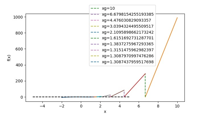
對於您選擇的多項式,您可以更改上述程式碼中所示的函式和導數多項式,並根據您的猜測值,您將獲得輸出。例如,如果您想找到 𝑥3−sin2(𝑥)−𝑥=0 的根,則在上述程式碼中,函式及其導數將更改為 -
# Function for f(x) and f'(x)
f=lambda x: x**3-(sin(x))**2-x
dfdx=lambda x: 3*x**2-2*sin(x)*cos(x)-1
然後對於 1 的猜測值,程式輸出將為 -
       xg           f(xg)
===========================
        1          -0.70807
     1.64919        1.84246
     1.39734        0.36083
     1.31747        0.0321
     1.30884        0.00036
     1.30874          0.0
===========================
Root 1.30874
並且,函式圖將如下所示 -
結論
在本教程中,您學習瞭如何使用牛頓-拉夫森方法求解方程的根。您還學習瞭如何在 pyplots 中繪製切線並顯示根的收斂。

2K+ 次瀏覽
