LightGBM - 迴歸

---

---

流行的機器學習方法 LightGBM（輕量級梯度提升機）用於迴歸和分類應用。當用於迴歸時，它會建立一系列決策樹，每棵樹都試圖透過減少前一棵樹的誤差來最小化損失函式（例如均方誤差）。

LightGBM 如何用於迴歸？

LightGBM 的基礎，梯度提升，按順序依次建立多個決策樹。每棵樹都努力糾正前一棵樹所犯的錯誤。

與其他按層增長樹的提升演算法不同，LightGBM 按葉節點增長樹。這意味著在擴充套件模型時，它會最佳化損失減少（即，最能改進模型的葉子節點）。這會產生更深、更準確的樹，但需要仔細調整以避免過擬合。

為了減少預期結果和實際結果之間的差異，LightGBM 使用兩種型別的迴歸任務損失函式——均方誤差 (MSE) 和平均絕對誤差 (MAE)。

何時使用 LightGBM 迴歸

以下是一些可以使用 LightGBM 進行迴歸的情況：

• 當給定大型資料集時。

• 當需要快速高效的模型時。

• 當您的資料包含大量特徵（列）或缺失值時。

使用 LightGBM 進行迴歸的示例

現在讓我們看看如何建立一個 LightGBM 迴歸模型。這些步驟將幫助您瞭解該過程的每個步驟是如何工作的。

步驟 1 - 安裝所需的庫

在開始之前，請確保您已安裝必要的庫。Scikit-learn 用於資料處理，lightgbm 用於 LightGBM 模型。

pip install pandas scikit-learn lightgbm

步驟 2 - 載入資料

首先，使用 pandas 載入資料集。此資料集包含與健康相關的資料，包括年齡、性別、BMI、子女數量、居住地、吸菸狀況和醫療費用。

import pandas as pd

# Load the dataset from your local file path
data = pd.read_csv('/My Docs/Python/medical_cost.csv')

# Display the first few rows of the dataset
print(data.head())

輸出

這將產生以下結果：

   age     sex     bmi  children smoker     region      charges
0   19  female  27.900         0    yes  southwest  16884.92400
1   18    male  33.770         1     no  southeast   1725.55230
2   28    male  33.000         3     no  southeast   4449.46200
3   33    male  22.705         0     no  northwest  21984.47061
4   32    male  28.880         0     no  northwest   3866.85520

步驟 3 - 分離特徵和目標變數

現在正在分離目標變數 (y) 和特徵 (X)。在本例中，我們希望使用其他特徵來預測“費用”列。

# 'charges' is the target column that we want to predict
# All columns except 'charges' are features
X = data.drop('charges', axis=1)  

# The 'charges' column is the target variable
y = data['charges']  

步驟 4 - 處理分類資料

資料集中的分類特徵（性別、吸菸者和地區）需要轉換為數值格式，因為 LightGBM 使用數值資料。獨熱編碼用於將這些類別列轉換為二進位制格式（0 和 1）。

# Convert categorical variables to numerical 
X = pd.get_dummies(X, drop_first=True)

這裡：

• pd.get_dummies() 用於為每個類別生成額外的二進位制列。

• drop_first=True 透過消除每個分類變數的第一個類別來避免多重共線性。

步驟 5 - 分割資料

為了瞭解模型的效能，我們將資料分成兩組——訓練集（佔資料的 80%）和測試集（佔資料的 20%）。

• train_test_split() 用於隨機分割資料，同時保持給定的比例 (test_size=0.2)。

• 使用 random_state = 42 可以確保分割結果可重現。

from sklearn.model_selection import train_test_split

# Split the data into training and test sets
X_train, X_test, y_train, y_test = train_test_split(X, y, test_size=0.2, random_state=42)

步驟 6：初始化 LightGBM 迴歸器

現在我們將為迴歸初始化 LightGBM 模型。LGBMRegressor 是 LightGBM 的實現，專門用於迴歸任務。LGBMRegressor 模型非常高效和靈活，可以有效地處理大型資料集。

from lightgbm import LGBMRegressor

# Initialize the LightGBM regressor model
model = LGBMRegressor()

步驟 7：訓練模型

接下來，我們將使用訓練資料 (X_train 和 y_train) 來訓練模型。這裡使用 fit() 方法透過查詢訓練資料中的模式並預測目標變數（費用）來訓練模型。

# Train the model on the training data
model.fit(X_train, y_train)

輸出

執行上述程式碼後，我們將得到以下結果：

[LightGBM] [Info] Auto-choosing col-wise multi-threading, the overhead of testing was 0.001000 seconds.
You can set `force_col_wise=true` to remove the overhead.
[LightGBM] [Info] Total Bins 319
[LightGBM] [Info] Number of data points in the train set: 1070, number of used features: 8
[LightGBM] [Info] Start training from score 13346.089733

 LGBMRegressori
LGBMRegressor()

步驟 8：進行預測

訓練後，我們使用模型對測試集 (X_test) 進行預測。model.predict(X_test) 根據從訓練資料中學習到的模式生成測試集的預測值。

# Predict on the test set
y_pred = model.predict(X_test)

步驟 9：評估模型

我們將使用均方誤差 (MSE) 來衡量模型的效能，這是一個常用的迴歸指標。均方誤差或 MSE 計算的是預期值和實際值之間的差異的平方平均值。較低的 MSE 值表示更好的效能。

from sklearn.metrics import mean_squared_error

# Calculate the MSE
mse = mean_squared_error(y_test, y_pred)
print(f'Mean Squared Error: {mse}')

輸出

這將生成以下輸出：

Mean Squared Error: 20557383.0620152

分析 MSE 值以瞭解模型預測目標變數的準確程度。如果 MSE 值很高，請考慮透過調整超引數或收集新資料來更新模型。

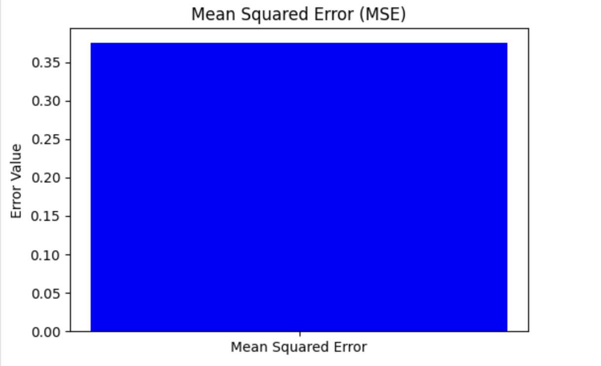
視覺化均方誤差 (MSE)

要檢視均方誤差，請使用 MSE 值建立一個條形圖。這提供了對問題嚴重程度的清晰直觀的表示。

這裡，您可以看到如何使用 matplotlib（一個流行的用於繪圖的 Python 庫）來繪製它：

import matplotlib.pyplot as plt
from sklearn.metrics import mean_squared_error

# Example data (replace these with your actual values)
# Actual values
y_test = [3, -0.5, 2, 7] 

# Predicted values
y_pred = [2.5, 0.0, 2, 8]  

# Calculate the MSE
mse = mean_squared_error(y_test, y_pred)

# Plotting the Mean Squared Error
plt.figure(figsize=(6, 4))
plt.bar(['Mean Squared Error'], [mse], color='blue')
plt.ylabel('Error Value')
plt.title('Mean Squared Error (MSE)')
plt.show()

輸出

以下是上述程式碼的結果：