- LightGBM 教程
- LightGBM - 首頁
- LightGBM - 概述
- LightGBM - 架構
- LightGBM - 安裝
- LightGBM - 核心引數
- LightGBM - Boosting演算法
- LightGBM - 樹生長策略
- LightGBM - 資料集結構
- LightGBM - 二元分類
- LightGBM - 迴歸
- LightGBM - 排序
- LightGBM - Python實現
- LightGBM - 引數調優
- LightGBM - 繪圖功能
- LightGBM - 早停訓練
- LightGBM - 特徵互動約束
- LightGBM 與其他Boosting演算法的比較
- LightGBM 有用資源
- LightGBM - 有用資源
- LightGBM - 討論
LightGBM - Python實現
本章將介紹使用Python開發LightGBM模型的步驟。我們將使用Scikit-learn的load_breast_cancer資料集構建一個二元分類模型。步驟如下:載入資料,準備LightGBM所需的資料,設定引數,訓練模型,進行預測,並評估結果。
LightGBM的實現
讓我們使用Python建立一個基本模型:
1. 載入資料集
首先,我們使用Scikit-learn的load_breast_cancer方法載入資料集。此資料集包含乳腺癌分類的特徵和標籤。
from sklearn.datasets import load_breast_cancer

# Load dataset
data = load_breast_cancer()
X = data.data
y = data.target
2. 分割資料
使用Scikit-learn的train_test_split方法將資料集分割成訓練集和測試集。這允許我們在一個數據集上訓練模型,然後在另一個數據集上評估其效能。
from sklearn.model_selection import train_test_split

# Split the data
X_train, X_test, y_train, y_test = train_test_split(X, y, test_size=0.2, random_state=42)
3. 準備LightGBM所需的資料
將訓練資料和測試資料轉換為LightGBM資料集格式。此步驟優化了LightGBM訓練演算法的資料格式。
import lightgbm as lgb

# Convert the data to LightGBM dataset format
train_data = lgb.Dataset(X_train, label=y_train)
test_data = lgb.Dataset(X_test, label=y_test, reference=train_data)
4. 定義引數
設定LightGBM模型的引數。這包括目標函式、評估指標、學習率、葉子節點數量和最大樹深度。
params = {
    'objective': 'binary',
    'metric': 'binary_logloss',
    'boosting_type': 'gbdt',
    'learning_rate': 0.1,
    # Increased from 31
    'num_leaves': 63,
    # Set to a positive value to limit depth
    'max_depth': 10
}
5. 訓練模型
使用訓練資料訓練LightGBM模型。為了防止過擬合,我們使用早停機制,這意味著當驗證集上沒有進展時訓練結束。
# Train the model with early stopping
lgb_model = lgb.train(
    params,
    train_data,
    num_boost_round=100,
    valid_sets=[test_data],
    # Use callback for early stopping
    callbacks=[lgb.early_stopping(stopping_rounds=10)]
)
輸出
以下是上述步驟的結果:
[LightGBM] [Info] Number of positive: 286, number of negative: 169
[LightGBM] [Info] Auto-choosing col-wise multi-threading, the overhead of testing was 0.000734 seconds.
You can set `force_col_wise=true` to remove the overhead.
[LightGBM] [Info] Total Bins 4548
[LightGBM] [Info] Number of data points in the train set: 455, number of used features: 30
[LightGBM] [Info] [binary:BoostFromScore]: pavg=0.628571 -> initscore=0.526093
[LightGBM] [Info] Start training from score 0.526093
[LightGBM] [Warning] No further splits with positive gain, best gain: -inf
[LightGBM] [Warning] No further splits with positive gain, best gain: -inf
6. 進行預測
使用訓練好的模型預測測試資料。我們將機率轉換為二元結果。
# Predict on the test set
y_pred = lgb_model.predict(X_test)
y_pred_binary = [1 if x > 0.5 else 0 for x in y_pred]
7. 評估模型
計算測試集的準確率分數以評估模型的效能。這使我們能夠了解模型對以前未見過的資料的效能。
from sklearn.metrics import accuracy_score

# Evaluate the model
accuracy = accuracy_score(y_test, y_pred_binary)
print(f"Accuracy: {accuracy:.2f}")
輸出
以下是上述模型的準確率:
Accuracy: 0.96
LightGBM模型的探索性資料分析 (EDA)
在訓練和測試LightGBM模型之前,必須進行探索性資料分析 (EDA),以瞭解資料集,識別模式並準備建模。EDA包括檢查資料集的結構、分佈、相關性和潛在問題。
以下是使用EDA處理load_breast_cancer資料集的步驟:
1. 載入和檢查資料集
首先,我們必須載入資料集並檢查其基本結構,例如樣本數量、特徵和目標變數。
import pandas as pd
from sklearn.datasets import load_breast_cancer

# Load dataset
data = load_breast_cancer()
df = pd.DataFrame(data.data, columns=data.feature_names)
df['target'] = data.target

# Inspect the dataset
print(df.head())
print(df.info())
print(df.describe())
輸出
這將產生以下結果:
   mean radius  mean texture  mean perimeter  mean area  mean smoothness  \
0        17.99         10.38          122.80     1001.0          0.11840
1        20.57         17.77          132.90     1326.0          0.08474
2        19.69         21.25          130.00     1203.0          0.10960
3        11.42         20.38           77.58      386.1          0.14250
4        20.29         14.34          135.10     1297.0          0.10030

   mean compactness  mean concavity  mean concave points  mean symmetry  \
0           0.27760          0.3001              0.14710         0.2419
1           0.07864          0.0869              0.07017         0.1812
2           0.15990          0.1974              0.12790         0.2069
3           0.28390          0.2414              0.10520         0.2597
4           0.13280          0.1980              0.10430         0.1809

   mean fractal dimension  ...  worst texture  worst perimeter  worst area  \
0                 0.07871  ...          17.33           184.60      2019.0
1                 0.05667  ...          23.41           158.80      1956.0
2                 0.05999  ...          25.53           152.50      1709.0
3                 0.09744  ...          26.50            98.87       567.7
4                 0.05883  ...          16.67           152.20      1575.0

   worst smoothness  worst compactness  worst concavity  worst concave points  \
0            0.1622             0.6656           0.7119                0.2654
1            0.1238             0.1866           0.2416                0.1860
2            0.1444             0.4245           0.4504                0.2430
3            0.2098             0.8663           0.6869                0.2575
4            0.1374             0.2050           0.4000                0.1625

   worst symmetry  worst fractal dimension  target
0          0.4601                  0.11890       0
1          0.2750                  0.08902       0
2          0.3613                  0.08758       0
3          0.6638                  0.17300       0
4          0.2364                  0.07678       0
2. 檢查缺失值
現在讓我們看看資料集中是否存在任何缺失值。
# Check for missing values
print(df.isnull().sum())
輸出
這將生成以下結果:
mean radius                0
mean texture               0
mean perimeter             0
mean area                  0
mean smoothness            0
mean compactness           0
mean concavity             0
mean concave points        0
mean symmetry              0
mean fractal dimension     0
radius error               0
texture error              0
perimeter error            0
area error                 0
smoothness error           0
compactness error          0
concavity error            0
concave points error       0
symmetry error             0
fractal dimension error    0
worst radius               0
worst texture              0
worst perimeter            0
worst area                 0
worst smoothness           0
worst compactness          0
worst concavity            0
worst concave points       0
worst symmetry             0
worst fractal dimension    0
target                     0
dtype: int64
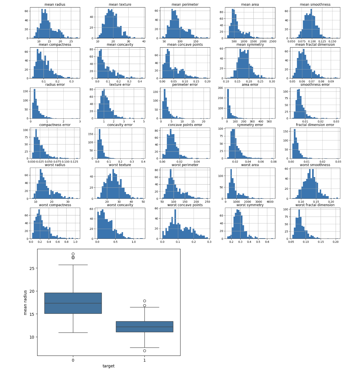
3. 特徵分佈
確定每個特徵的分佈。為了更多地瞭解特徵值的範圍和分佈,可以使用直方圖、箱線圖或其他視覺化方法。
import matplotlib.pyplot as plt
import seaborn as sns

# Plot histograms for each feature
df.iloc[:, :-1].hist(bins=30, figsize=(20, 15))
plt.show()

# Box plot for a selected feature
sns.boxplot(x='target', y='mean radius', data=df)
plt.show()
輸出
這將建立以下結果:
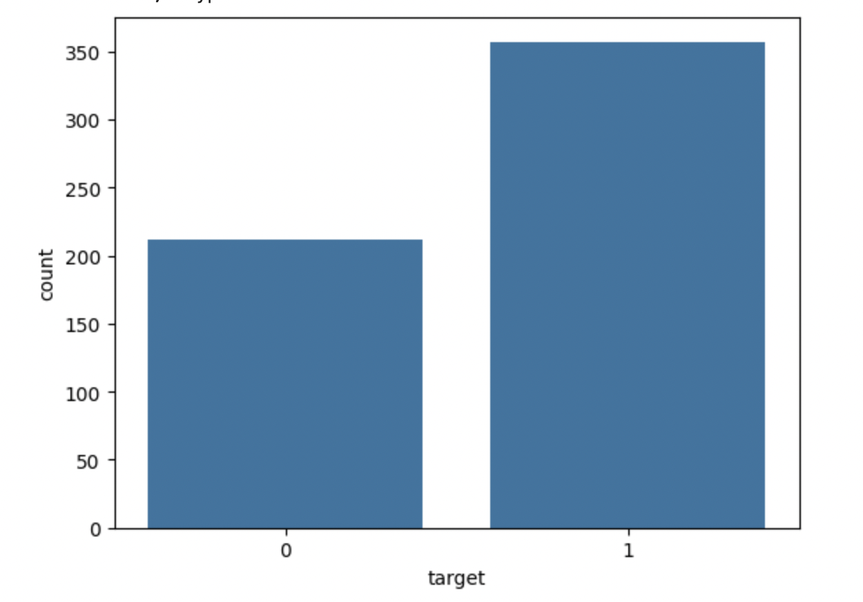
4. 分析類別分佈
檢查目標變數的分佈以查詢類別平衡。這將使您能夠識別資料集是否不平衡。
# Class distribution
print(df['target'].value_counts())
sns.countplot(x='target', data=df)
plt.show()
輸出
這將顯示以下輸出:
target
1    357
0    212
Name: count, dtype: int64
總結
按照這些步驟,您可以建立和測試用於Python中分類問題的LightGBM模型。可以透過根據需要調整引數和準備步驟,將此技術修改為適用於不同的資料集和問題。