- LightGBM 教程
- LightGBM - 首頁
- LightGBM - 概述
- LightGBM - 架構
- LightGBM - 安裝
- LightGBM - 核心引數
- LightGBM - Boosting 演算法
- LightGBM - 樹生長策略
- LightGBM - 資料集結構
- LightGBM - 二元分類
- LightGBM - 迴歸
- LightGBM - 排序
- LightGBM - Python 實現
- LightGBM - 引數調整
- LightGBM - 繪圖功能
- LightGBM - 早停訓練
- LightGBM - 特徵互動約束
- LightGBM 與其他 Boosting 演算法的比較
- LightGBM 有用資源
- LightGBM - 有用資源
- LightGBM - 討論
LightGBM - 繪圖功能
LightGBM 提供各種建立繪圖的工具,幫助您視覺化模型的效能、特徵重要性等。因此,在本章中,我們將編寫一些您可以與 LightGBM 一起使用的常用繪圖函式。
LightGBM 繪圖函式
以下是 LightGBM 中常用的繪圖函式列表:
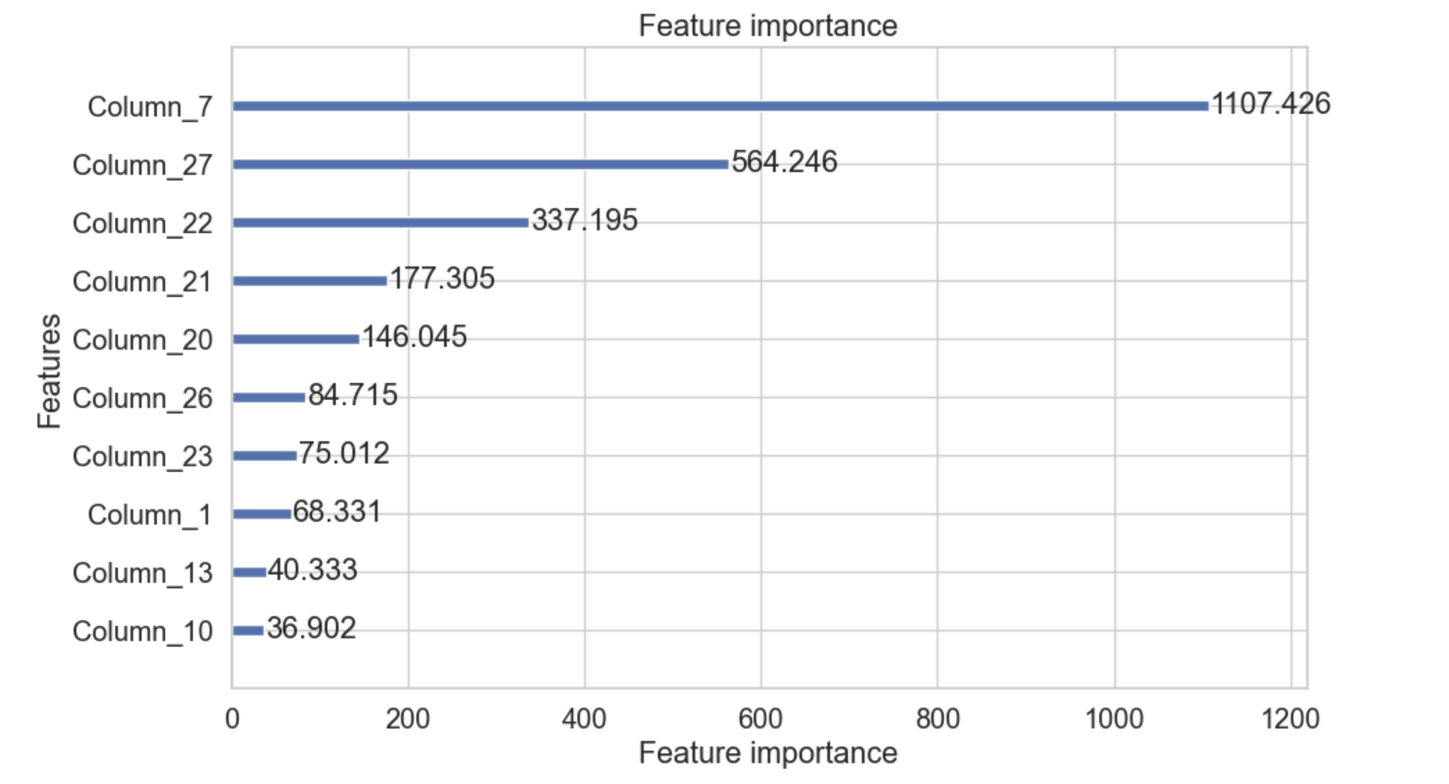
plot_importance()
plot_importance() 方法使用增強器物件,然後繪製特徵重要性。此方法使用名為 importance_type 的引數,該引數用於設定為字串“split”,它將繪製特徵用於分割的次數,當設定為字串“gain”時,它將繪製分割的增益。引數 importance_type 的值為“split”。
該函式還有一個名為 max_num_features 的引數,它接受一個整數,表示我們需要在圖中包含多少個特徵。我們也可以藉助此引數來限制特徵的數量。
語法
以下是我們可以用於 plot_importance() 函式的語法:
lightgbm.plot_importance(
   ax=None,
   booster,
   height=0.2,
   ylim=None,
   xlim=None,
   xlabel='Feature importance',
   title='Feature importance',
   importance_type='split',
   ylabel='Features',
   ignore_zero=True,
   max_num_features=None,
   grid=True,
   figsize=None,
   precision=3
)
引數
以下是使用 plot_importance() 函式所需的引數:
booster − 它是訓練好的 LightGBM 模型。
importance_type − 用於定義如何計算特徵重要性。它有兩個值:“split”和“gain”。預設值為“split”。
max_num_features − 用於限制頂級特徵的數量。
figsize − 它是一個元組,用於顯示繪圖的大小,例如 (10, 6)。
xlabel, ylabel − 這些是 x 軸和 y 軸的標籤。
title − 它定義了繪圖的標題。
ignore_zero − 如果設定為 True,它基本上會忽略重要性為零的特徵。
grid − 如果設定為 True,則它會在繪圖中顯示網格。
示例
以下示例演示了 plot_importance() 函式的用法:
import lightgbm as lgb
import matplotlib.pyplot as plt

# Assuming you have a trained model `gbm`
lgb.plot_importance(gbm, importance_type='gain', max_num_features=10, figsize=(10, 6))
plt.show()
輸出
以下是上述程式碼的輸出:
plot_metric()
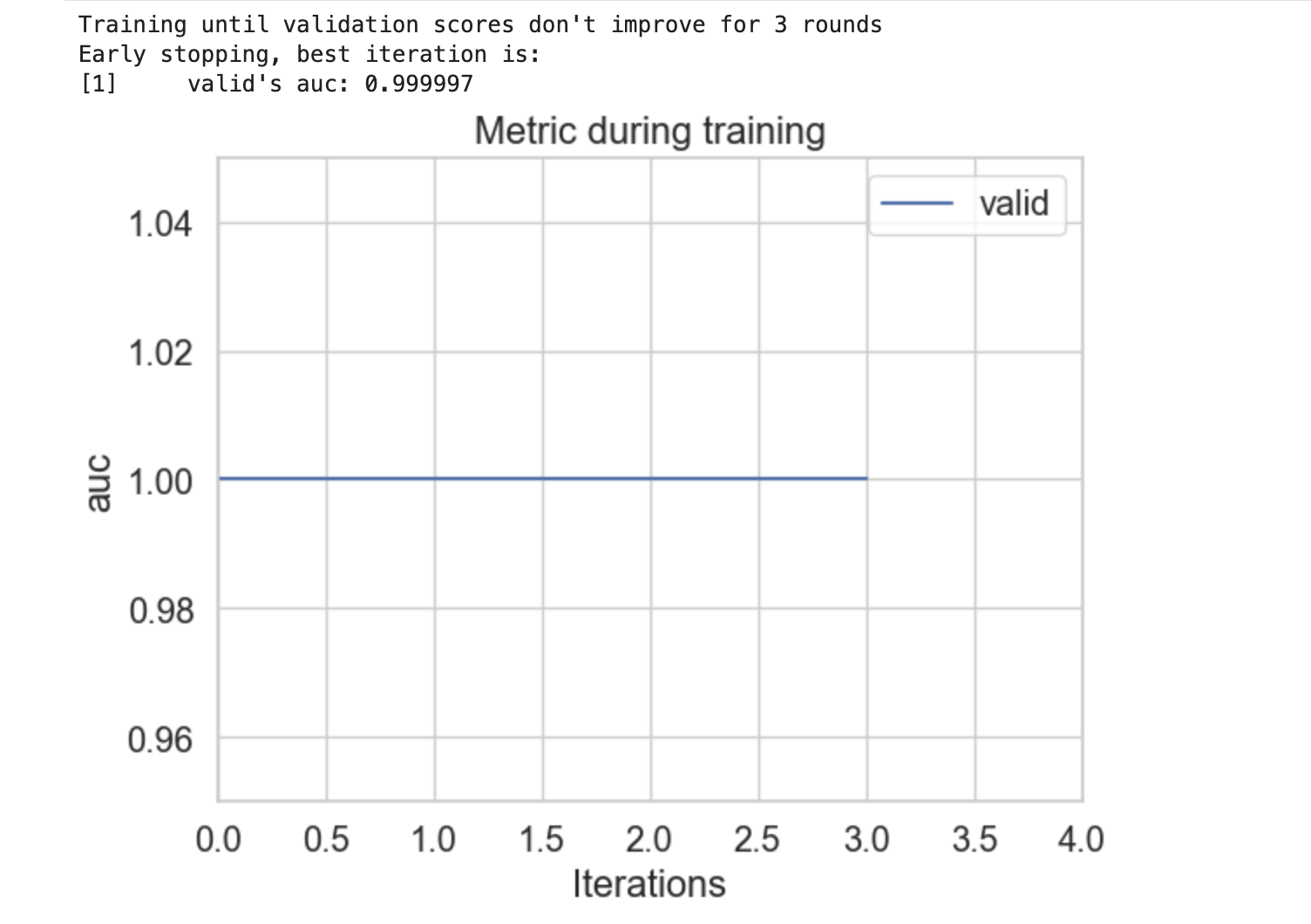
plot_metric() 函式用於繪製評估指標的結果。要使用此函式,我們必須在方法中提供一個增強器物件才能繪製在資料集上評估的評估指標。
語法
以下是我們可以用於 plot_metric() 函式的語法:
lightgbm.plot_metric(
   eval_result,
   metric=None,
   dataset_names=None,
   ax=None,
   title='Metric during training',
   xlabel='Iterations',
   ylabel='Auto',
   figsize=None,
   grid=True
)
引數
以下是 plot_metric() 函式所需的引數:
eval_result − 它是由 train() 方法返回的字典。它基本上包含評估結果。
metric − 您要繪製的評估指標。它是 None,因此會繪製所有指標。
dataset_names − 用於繪圖的資料集名稱列表。
ax − 用於繪圖的 Matplotlib 軸物件。如果設定為 None,則會建立一個新的繪圖。
title − 繪圖的標題。
xlabel − X 軸的標籤。
ylabel − Y 軸的標籤。
figsize − 影像大小的元組。
grid − 用於顯示網格。其預設值為 True。
示例
以下是使用模型並顯示 plot_metric() 函式用法的完整 Python 程式碼:
import lightgbm as lgb
import matplotlib.pyplot as plt
from sklearn.datasets import make_blobs
from sklearn.model_selection import train_test_split

# Generate sample binary classification data
X, y = make_blobs(n_samples=10_000, centers=2)

# Split the data
X_train, X_valid, y_train, y_valid = train_test_split(X, y, train_size=0.8)

# Prepare the dataset for LightGBM
dtrain = lgb.Dataset(X_train, label=y_train)
dvalid = lgb.Dataset(X_valid, label=y_valid)

# Dictionary to store results
evals_result = {}

# Train the model
model = lgb.train(
   params={
      "objective": "binary",
      "metric": "auc",
   },
   train_set=dtrain,
   valid_sets=[dvalid],
   valid_names=['valid'],
   num_boost_round=10,
   callbacks=[
      lgb.early_stopping(stopping_rounds=3),
      lgb.record_evaluation(evals_result)
   ]
)

# Plot the evaluation metric
lgb.plot_metric(evals_result, metric='auc')
plt.show()
輸出
以下是上述程式碼的結果:
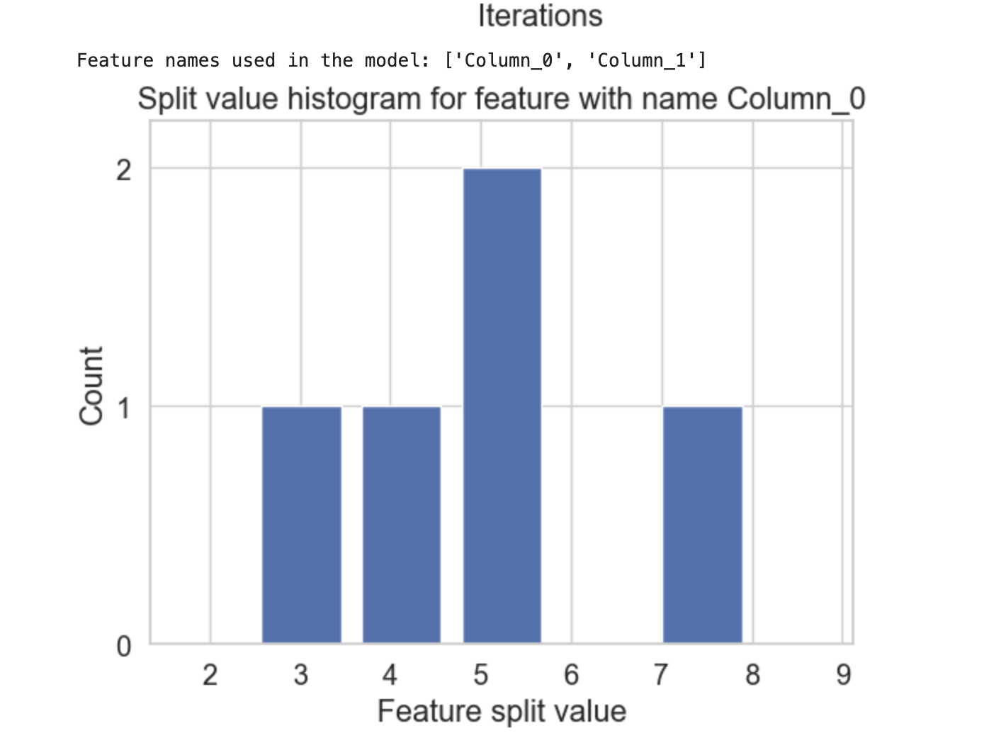
plot_split_value_histogram()
plot_split_value_histogram() 函式基本上接受輸入增強器物件和特徵名稱/索引。之後,它會為給定的特徵繪製分割值直方圖。
語法
以下是您可以用於 plot_split_value_histogram() 函式的語法:
lightgbm.plot_split_value_histogram(
   booster,
   feature,
   bins=100,
   ax=None,
   width_coef=0.8,
   xlim=None,
   ylim=None,
   title=None,
   xlabel=None,
   ylabel=None,
   figsize=None,
   dpi=None,
   grid=False,
)
引數
以下是 plot_split_value_histogram() 函式的必需和可選引數
booster − 它是訓練好的 LightGBM 模型,也稱為增強器物件。
feature − 您要繪製的特徵的名稱。
bins − 您可以用於直方圖的箱數。
ax − 它是可選的 Matplotlib 軸物件。如果給出,則繪圖將繪製在此軸上。
width_coef − 用於管理直方圖中條形寬度係數。
xlim − x 軸限制的元組。
ylim − y 軸限制的元組。
title − 繪圖的標題。
xlabel − x 軸的標籤。
ylabel − y 軸的標籤。
figsize − 影像大小的元組。
dpi − 繪圖的每英寸點數。
grid − 此引數使用布林值在繪圖中顯示網格。
示例
以下是如何包含 plot_split_value_histogram() 函式並檢視結果的方法:
# Complete code is similar to the above mentioned example for plot_metric()
# Plot the split value histogram
lgb.plot_split_value_histogram(model, feature=feature_to_plot)
plt.show()
輸出
這將建立以下結果
plot_tree()
plot_tree() 函式允許您繪製整合中的單個樹。為此,我們必須提到一個增強器物件以及我們要繪製的樹的索引。
語法
以下是您可以用於 plot_split_value_histogram() 函式的語法:
lightgbm.plot_tree(
   booster,
   tree_index=0,
   figsize=(10, 10),
   dpi=None,
   show_info=True,
   precision=3,
   orientation='horizontal',
   example_case=None,
)
引數
以下是 plot_split_value_histogram() 函式的必需和可選引數
booster − 要繪製的增強器或 LGBMModel 物件。
tree_index − 目標軸物件。如果為 None,則建立新的圖形和軸。
figsize − 要繪製的目標樹的索引。
dpi − 影像的解析度。
show_info − 用於顯示有關樹中每個節點的附加資訊。
precision − 用於將浮點值的顯示限制在一定的精度。
orientation − 樹的方向。其值可以是水平或垂直。
example_case − 與訓練資料具有相同結構的單行。
create_tree_digraph()
create_tree_digraph() 方法用於顯示來自 LightGBM 模型的給定決策樹的結構。它基本上會生成一個圖,顯示樹在每個節點如何分割資料,這使得更容易理解模型的決策過程。
語法
以下是您可以用於 create_tree_digraph() 函式的語法:
lightgbm.create_tree_digraph(
   booster,
   tree_index=0,
   show_info=None,
   precision=3,
   orientation='horizontal',
   example_case=None,
   max_category_values=10
)
引數
以下是 create_tree_digraph() 函式的必需和可選引數
booster − 要轉換的增強器或 LGBMModel 物件。
tree_index − 要轉換的目標樹的索引。
show_info − 應在節點中顯示的資訊。值可以是 split_gain、internal_value、internal_count、internal_weight、leaf_count、leaf_weight 和 data_percentage。
precision − 用於將浮點值的顯示限制在特定精度。
orientation − 樹的方向。值可以是水平或垂直。
example_case − 與訓練資料具有相同結構的單行。
max_category_values − 要在樹節點中顯示的最大類別值數。如果閾值的值大於此值,它將被摺疊並在標籤工具提示中顯示。