Python深度學習 - 實現

---

---

在這個深度學習實現中，我們的目標是預測某家銀行的客戶流失或流轉資料——哪些客戶可能離開這家銀行的服務。所使用的資料集相對較小，包含10000行和14列。我們使用Anaconda發行版以及Theano、TensorFlow和Keras等框架。Keras構建在Tensorflow和Theano之上，它們充當Keras的後端。

# Artificial Neural Network
# Installing Theano
pip install --upgrade theano

# Installing Tensorflow
pip install –upgrade tensorflow

# Installing Keras
pip install --upgrade keras

步驟1：資料預處理

In[]:

# Importing the libraries
   import numpy as np
   import matplotlib.pyplot as plt
   import pandas as pd
 
# Importing the database
   dataset = pd.read_csv('Churn_Modelling.csv')

步驟2

我們建立資料集特徵矩陣和目標變數矩陣，目標變數是第14列，標記為“Exited”。

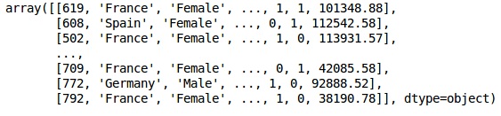
資料的初始外觀如下所示：

In[]:
X = dataset.iloc[:, 3:13].values
Y = dataset.iloc[:, 13].values
X

輸出

步驟3

Y

輸出

array([1, 0, 1, ..., 1, 1, 0], dtype = int64)

步驟4

我們透過編碼字串變數來簡化分析。我們使用ScikitLearn函式“LabelEncoder”自動將各列中的不同標籤編碼為0到n_classes-1之間的值。

from sklearn.preprocessing import LabelEncoder, OneHotEncoder
labelencoder_X_1 = LabelEncoder() 
X[:,1] = labelencoder_X_1.fit_transform(X[:,1]) 
labelencoder_X_2 = LabelEncoder() 
X[:, 2] = labelencoder_X_2.fit_transform(X[:, 2])
X

輸出

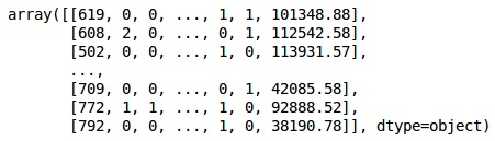
在上面的輸出中，國家名稱被替換為0、1和2；而男性和女性分別被替換為0和1。

步驟5

標籤編碼資料

我們使用相同的ScikitLearn庫和另一個名為OneHotEncoder的函式來傳遞列號，從而建立一個虛擬變數。

onehotencoder = OneHotEncoder(categorical features = [1])
X = onehotencoder.fit_transform(X).toarray()
X = X[:, 1:]
X

現在，前兩列表示國家，第四列表示性別。

輸出

我們總是將資料分成訓練集和測試集；我們在訓練資料上訓練模型，然後在測試資料上檢查模型的準確性，這有助於評估模型的效率。

步驟6

我們使用ScikitLearn的train_test_split函式將我們的資料分成訓練集和測試集。我們將訓練集與測試集的比例保持為80:20。

#Splitting the dataset into the Training set and the Test Set
from sklearn.model_selection import train_test_split
X_train, X_test, y_train, y_test = train_test_split(X, y, test_size = 0.2)

有些變數的值以千計，而有些變數的值只有幾十或幾。我們對資料進行縮放，使其更具代表性。

步驟7

在這段程式碼中，我們使用StandardScaler函式擬合併轉換訓練資料。我們標準化縮放，以便使用相同的擬合方法來轉換/縮放測試資料。

# Feature Scaling

fromsklearn.preprocessing import StandardScaler 
sc = StandardScaler() 
X_train = sc.fit_transform(X_train) 
X_test = sc.transform(X_test)

輸出

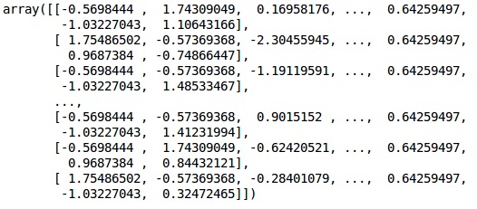
資料現在已正確縮放。最後，我們完成了資料預處理。現在，我們將開始構建我們的模型。

步驟8

我們在這裡匯入所需的模組。我們需要Sequential模組來初始化神經網路，以及dense模組來新增隱藏層。

# Importing the Keras libraries and packages 
import keras 
from keras.models import Sequential 
from keras.layers import Dense

步驟9

我們將模型命名為Classifier，因為我們的目標是分類客戶流失。然後我們使用Sequential模組進行初始化。

#Initializing Neural Network 
classifier = Sequential()

步驟10

我們使用dense函式逐一新增隱藏層。在下面的程式碼中，我們將看到許多引數。

我們的第一個引數是output_dim。這是我們新增到此層中的節點數。init是隨機梯度下降的初始化。在神經網路中，我們為每個節點分配權重。在初始化時，權重應該接近於零，我們使用uniform函式隨機初始化權重。input_dim引數僅在第一層需要，因為模型不知道我們的輸入變數的數量。這裡輸入變數的總數是11。在第二層中，模型會自動從第一隱藏層知道輸入變數的數量。

執行以下程式碼行以新增輸入層和第一隱藏層：

classifier.add(Dense(units = 6, kernel_initializer = 'uniform', 
activation = 'relu', input_dim = 11))

執行以下程式碼行以新增第二隱藏層：

classifier.add(Dense(units = 6, kernel_initializer = 'uniform', 
activation = 'relu'))

執行以下程式碼行以新增輸出層：

classifier.add(Dense(units = 1, kernel_initializer = 'uniform', 
activation = 'sigmoid'))

步驟11

編譯ANN

到目前為止，我們已經向分類器添加了多層。我們現在將使用compile方法編譯它們。在最終編譯中新增的引數控制著整個神經網路，因此我們必須小心這一步。

以下是引數的簡要說明。

第一個引數是Optimizer。這是一種用於尋找最優權重集的演算法。這種演算法稱為隨機梯度下降 (SGD)。在這裡，我們使用幾種型別中的一種，稱為“Adam最佳化器”。SGD取決於損失，因此我們的第二個引數是損失。如果我們的因變數是二元的，我們使用稱為‘binary_crossentropy’的對數損失函式；如果我們的因變數在輸出中有多於兩個類別，則我們使用‘categorical_crossentropy’。我們希望根據accuracy來提高神經網路的效能，因此我們新增metrics作為準確性。

# Compiling Neural Network 
classifier.compile(optimizer = 'adam', loss = 'binary_crossentropy', metrics = ['accuracy'])

步驟12

此步驟需要執行多行程式碼。

將ANN擬合到訓練集

我們現在在訓練資料上訓練我們的模型。我們使用fit方法來擬合我們的模型。我們還最佳化權重以提高模型效率。為此，我們必須更新權重。Batch size是在更新權重之後觀測值的數量。Epoch是迭代的總數。批次大小和時期值是透過反覆試驗的方法選擇的。

classifier.fit(X_train, y_train, batch_size = 10, epochs = 50)

進行預測和評估模型

# Predicting the Test set results
y_pred = classifier.predict(X_test)
y_pred = (y_pred > 0.5)

預測單個新的觀測值

# Predicting a single new observation
"""Our goal is to predict if the customer with the following data will leave the bank:
Geography: Spain
Credit Score: 500
Gender: Female
Age: 40
Tenure: 3
Balance: 50000
Number of Products: 2
Has Credit Card: Yes
Is Active Member: Yes

步驟13

預測測試集結果

預測結果將給出客戶離開公司的機率。我們將把該機率轉換為二進位制0和1。

# Predicting the Test set results 
y_pred = classifier.predict(X_test) 
y_pred = (y_pred > 0.5)

new_prediction = classifier.predict(sc.transform
(np.array([[0.0, 0, 500, 1, 40, 3, 50000, 2, 1, 1, 40000]])))
new_prediction = (new_prediction > 0.5)

步驟14

這是我們評估模型效能的最後一步。我們已經有了原始結果，因此我們可以構建混淆矩陣來檢查模型的準確性。

製作混淆矩陣

from sklearn.metrics import confusion_matrix
cm = confusion_matrix(y_test, y_pred)
print (cm)

輸出

loss: 0.3384 acc: 0.8605
[ [1541 54]
[230 175] ]

根據混淆矩陣，我們可以計算模型的準確率為：

Accuracy = 1541+175/2000=0.858

我們達到了85.8%的準確率，這很好。

前向傳播演算法

在本節中，我們將學習如何編寫程式碼來對簡單的神經網路進行前向傳播（預測）：

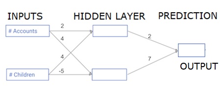
每個資料點都是一個客戶。第一個輸入是他們有多少個賬戶，第二個輸入是他們有多少個孩子。該模型將預測使用者明年將進行多少筆交易。

輸入資料預載入為input_data，權重在一個名為weights的字典中。隱藏層中第一個節點的權重陣列位於weights['node_0']中，隱藏層中第二個節點的權重陣列位於weights['node_1']中。

饋送到輸出節點的權重在weights中可用。

修正線性啟用函式

“啟用函式”是在每個節點工作的函式。它將節點的輸入轉換為某種輸出。

修正線性啟用函式（稱為ReLU）廣泛用於非常高效能的網路。此函式以單個數字作為輸入，如果輸入為負，則返回0；如果輸入為正，則返回輸入作為輸出。

以下是一些示例：

• relu(4) = 4
• relu(-2) = 0

我們填寫relu()函式的定義：

• 我們使用max()函式來計算relu()的輸出值。
• 我們應用relu()函式到node_0_input來計算node_0_output。
• 我們應用relu()函式到node_1_input來計算node_1_output。

import numpy as np
input_data = np.array([-1, 2])
weights = {
   'node_0': np.array([3, 3]),
   'node_1': np.array([1, 5]),
   'output': np.array([2, -1])
}
node_0_input = (input_data * weights['node_0']).sum()
node_0_output = np.tanh(node_0_input)
node_1_input = (input_data * weights['node_1']).sum()
node_1_output = np.tanh(node_1_input)
hidden_layer_output = np.array(node_0_output, node_1_output)
output =(hidden_layer_output * weights['output']).sum()
print(output)

def relu(input):
   '''Define your relu activation function here'''
   # Calculate the value for the output of the relu function: output
   output = max(input,0)
      # Return the value just calculated
   return(output)
# Calculate node 0 value: node_0_output
node_0_input = (input_data * weights['node_0']).sum()
node_0_output = relu(node_0_input)

# Calculate node 1 value: node_1_output
node_1_input = (input_data * weights['node_1']).sum()
node_1_output = relu(node_1_input)

# Put node values into array: hidden_layer_outputs
hidden_layer_outputs = np.array([node_0_output, node_1_output])

# Calculate model output (do not apply relu)
odel_output = (hidden_layer_outputs * weights['output']).sum()
print(model_output)# Print model output

輸出

0.9950547536867305
-3

將網路應用於許多觀測值/資料行

在本節中，我們將學習如何定義一個名為predict_with_network()的函式。此函式將為從上面網路中獲取的多個數據觀測值（作為input_data）生成預測。使用上面網路中給出的權重。relu()函式定義也正在使用。

讓我們定義一個名為predict_with_network()的函式，它接受兩個引數 - input_data_row和weights - 並返回網路的預測作為輸出。

我們計算每個節點的輸入值和輸出值，並將它們儲存為：node_0_input、node_0_output、node_1_input和node_1_output。

為了計算節點的輸入值，我們將相關的陣列相乘並計算它們的總和。

為了計算節點的輸出值，我們將relu()函式應用於節點的輸入值。我們使用“for迴圈”來迭代input_data：

我們還使用我們的predict_with_network()為input_data的每一行 - input_data_row生成預測。我們還將每個預測新增到results中。

# Define predict_with_network()
def predict_with_network(input_data_row, weights):
   # Calculate node 0 value
   node_0_input = (input_data_row * weights['node_0']).sum()
   node_0_output = relu(node_0_input)
   
   # Calculate node 1 value
   node_1_input = (input_data_row * weights['node_1']).sum()
   node_1_output = relu(node_1_input)
   
   # Put node values into array: hidden_layer_outputs
   hidden_layer_outputs = np.array([node_0_output, node_1_output])
   
   # Calculate model output
   input_to_final_layer = (hidden_layer_outputs*weights['output']).sum()
   model_output = relu(input_to_final_layer)
# Return model output
   return(model_output)

# Create empty list to store prediction results
results = []
for input_data_row in input_data:
   # Append prediction to results
   results.append(predict_with_network(input_data_row, weights))
print(results)# Print results

輸出

[0, 12]

在這裡，我們使用了relu函式，其中relu(26) = 26，relu(-13)=0，依此類推。

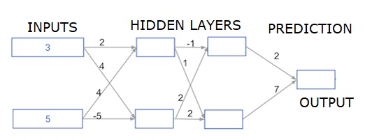
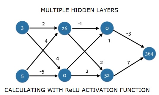
深度多層神經網路

在這裡，我們編寫程式碼來對具有兩個隱藏層的神經網路進行前向傳播。每個隱藏層都有兩個節點。輸入資料已預載入為input_data。第一個隱藏層中的節點稱為node_0_0和node_0_1。

它們的權重分別預載入為weights['node_0_0']和weights['node_0_1']。

第二個隱藏層中的節點稱為node_1_0和node_1_1。它們的權重分別預載入為weights['node_1_0']和weights['node_1_1']。

然後，我們使用預載入為weights['output']的權重建立來自隱藏節點的模型輸出。

我們使用其權重weights['node_0_0']和給定的input_data計算node_0_0_input。然後應用relu()函式以獲得node_0_0_output。

我們對node_0_1_input執行與上述相同的操作以獲得node_0_1_output。

我們使用其權重weights['node_1_0']和第一隱藏層的輸出 - hidden_0_outputs計算node_1_0_input。然後應用relu()函式以獲得node_1_0_output。

我們對node_1_1_input執行與上述相同的操作以獲得node_1_1_output。

我們使用weights['output']和第二隱藏層的輸出hidden_1_outputs陣列計算model_output。我們不將relu()函式應用於此輸出。

import numpy as np
input_data = np.array([3, 5])
weights = {
   'node_0_0': np.array([2, 4]),
   'node_0_1': np.array([4, -5]),
   'node_1_0': np.array([-1, 1]),
   'node_1_1': np.array([2, 2]),
   'output': np.array([2, 7])
}
def predict_with_network(input_data):
   # Calculate node 0 in the first hidden layer
   node_0_0_input = (input_data * weights['node_0_0']).sum()
   node_0_0_output = relu(node_0_0_input)
   
   # Calculate node 1 in the first hidden layer
   node_0_1_input = (input_data*weights['node_0_1']).sum()
   node_0_1_output = relu(node_0_1_input)
   
   # Put node values into array: hidden_0_outputs
   hidden_0_outputs = np.array([node_0_0_output, node_0_1_output])
   
   # Calculate node 0 in the second hidden layer
   node_1_0_input = (hidden_0_outputs*weights['node_1_0']).sum()
   node_1_0_output = relu(node_1_0_input)
   
   # Calculate node 1 in the second hidden layer
   node_1_1_input = (hidden_0_outputs*weights['node_1_1']).sum()
   node_1_1_output = relu(node_1_1_input)
   
   # Put node values into array: hidden_1_outputs
   hidden_1_outputs = np.array([node_1_0_output, node_1_1_output])
   
   # Calculate model output: model_output
   model_output = (hidden_1_outputs*weights['output']).sum()
      # Return model_output
   return(model_output)
output = predict_with_network(input_data)
print(output)

輸出

364