
 資料結構
資料結構 網路
網路 RDBMS
RDBMS 作業系統
作業系統 Java
Java iOS
iOS HTML
HTML CSS
CSS Android
 Python
 C 程式設計
 C++
C++ C#
C# MongoDB
 MySQL
MySQL Javascript
 PHP
PHP使用 PyTorch 進行線性迴歸?
線性迴歸簡介
簡單的線性迴歸基礎
它讓我們理解兩個連續變數之間的關係。
示例 −
x = 自變數
體重
y = 因變數
身高
y = αx + β
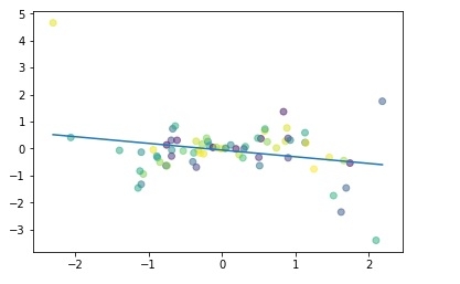
讓我們透過一個程式瞭解簡單的線性迴歸 −
#Simple linear regression

import numpy as np
import matplotlib.pyplot as plt

np.random.seed(1)
n = 70
x = np.random.randn(n)
y = x * np.random.randn(n)

colors = np.random.rand(n)
plt.plot(np.unique(x), np.poly1d(np.polyfit(x, y, 1))(np.unique(x)))

plt.scatter(x, y, c = colors, alpha = 0.5)
plt.show()
輸出
線性迴歸的用途
最大程度地減少點和線 (y = αx + β) 之間的距離
調整
係數:α
切點/偏差:β
使用 PyTorch 構建線性迴歸模型
假設我們的係數 (α) 為 2,切點 (β) 為 1,則我們的方程將變為 −
y = 2x +1 # 線性模型
構建資料集
x_values = [i for i in range(11)]
x_values
輸出
[0, 1, 2, 3, 4, 5, 6, 7, 8, 9, 10]
# 轉換為 numpy
x_train = np.array(x_values, dtype = np.float32)
x_train.shape
輸出
(11,)
#Important: 2D required
x_train = x_train.reshape(-1, 1)
x_train.shape
輸出
(11, 1)
y_values = [2*i + 1 for i in x_values]
y_values
輸出
[1, 3, 5, 7, 9, 11, 13, 15, 17, 19, 21]
#list iteration

y_values = []
for i in x_values:
result = 2*i +1
y_values.append(result)

y_values
輸出
[1, 3, 5, 7, 9, 11, 13, 15, 17, 19, 21]
y_train = np.array(y_values, dtype = np.float32)
y_train.shape
輸出
(11,)
#2D required
y_train = y_train.reshape(-1, 1)
y_train.shape
輸出
(11, 1)
構建模型
#import libraries
import torch
import torch.nn as nn
from torch.autograd import Variable

#Create Model class
class LinearRegModel(nn.Module):
def __init__(self, input_size, output_size):
super(LinearRegModel, self).__init__()
self.linear = nn.Linear(input_dim, output_dim)

def forward(self, x):
out = self.linear(x)
return out

input_dim = 1
output_dim = 1

model = LinearRegModel(input_dim, output_dim)

criterion = nn.MSELoss()

learning_rate = 0.01
optimizer = torch.optim.SGD(model.parameters(), lr = learning_rate)

epochs = 100
for epoch in range(epochs):
epoch += 1
#convert numpy array to torch variable
inputs = Variable(torch.from_numpy(x_train))
labels = Variable(torch.from_numpy(y_train))

#Clear gradients w.r.t parameters
optimizer.zero_grad()

#Forward to get output
outputs = model.forward(inputs)

#Calculate Loss
loss = criterion(outputs, labels)

#Getting gradients w.r.t parameters
loss.backward()

#Updating parameters
optimizer.step()

print('epoch {}, loss {}'.format(epoch, loss.data[0]))
輸出
epoch 1, loss 276.7417907714844
epoch 2, loss 22.601360321044922
epoch 3, loss 1.8716105222702026
epoch 4, loss 0.18043726682662964
epoch 5, loss 0.04218350350856781
epoch 6, loss 0.03060017339885235
epoch 7, loss 0.02935197949409485
epoch 8, loss 0.02895027957856655
epoch 9, loss 0.028620922937989235
epoch 10, loss 0.02830091118812561
......
......
epoch 94, loss 0.011018744669854641
epoch 95, loss 0.010895680636167526
epoch 96, loss 0.010774039663374424
epoch 97, loss 0.010653747245669365
epoch 98, loss 0.010534750297665596
epoch 99, loss 0.010417098179459572
epoch 100, loss 0.010300817899405956
因此,我們可以看出從第 1 個曆元到第 100 個曆元,損失已大幅減少。
繪製圖形
#Purely inference
predicted = model(Variable(torch.from_numpy(x_train))).data.numpy()
predicted
y_train

#Plot Graph

#Clear figure
plt.clf()

#Get predictions
predicted = model(Variable(torch.from_numpy(x_train))).data.numpy()

#Plot true data
plt.plot(x_train, y_train, 'go', label ='True data', alpha = 0.5)

#Plot predictions
plt.plot(x_train, predicted, '--', label='Predictions', alpha = 0.5)

#Legend and Plot
plt.legend(loc = 'best')
plt.show()
輸出
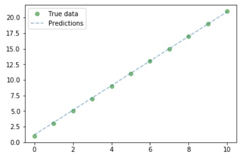
因此,我們可以從圖形中看出我們的真實值和預測值非常相似。

更新於: 2019 年 7 月 30 日
493 次瀏覽

廣告