
 資料結構
資料結構 網路
網路 關係型資料庫管理系統
 作業系統
作業系統 Java
Java iOS
iOS HTML
HTML CSS
CSS Android
 Python
 C 語言程式設計
 C++
C++ C#
C# MongoDB
 MySQL
MySQL Javascript
 PHP
PHP如何使用 OpenCV Python 比較兩張影像的直方圖?
可以使用 **cv2.compareHist()** 函式比較兩張影像的直方圖。**cv2.compareHist()** 函式接受三個輸入引數 - **hist1、hist2** 和 **compare_method**。**hist1** 和 **hist2** 是兩張輸入影像的直方圖,**compare_method** 是用於計算直方圖之間匹配程度的度量標準。它返回一個數值引數,表示兩個直方圖彼此匹配的程度。有四種可用的度量標準來比較直方圖 - 相關性、卡方、交集和巴氏距離。
步驟
要比較兩張影像的直方圖,可以按照以下步驟操作:
匯入所需的庫。在以下所有 Python 示例中,所需的 Python 庫是 **OpenCV** 和 **Matplotlib**。請確保您已安裝它們。
使用 **cv2.imread()** 函式讀取輸入影像。傳遞輸入影像的完整路徑。
使用 **cv2.calcHist()** 計算兩張輸入影像的直方圖。
使用 **cv2.normalize()** 對上面計算的兩張輸入影像的直方圖進行歸一化。
使用 **cv2.compareHist()** 比較這些歸一化後的直方圖。它返回比較度量值。將合適的直方圖比較方法作為引數傳遞給此方法。
列印直方圖比較度量值。可以選擇繪製兩個直方圖以進行視覺理解。
讓我們看一些示例,以便更清楚地瞭解問題。
輸入影像
我們將在下面的示例中使用以下影像作為輸入檔案。


示例
在此示例中,我們比較兩張輸入影像的直方圖。我們計算並歸一化兩張影像的直方圖,然後比較這些歸一化後的直方圖。
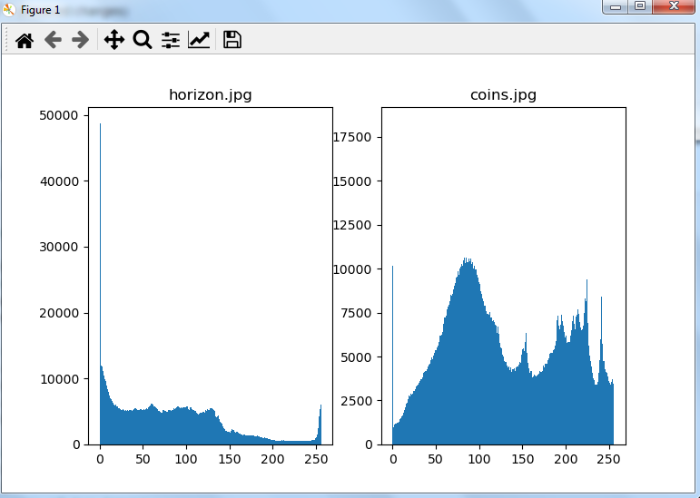
# import required libraries
import cv2
import matplotlib.pyplot as plt

# Load the images
img1 = cv2.imread('horizon.jpg')
img2 = cv2.imread('coins.jpg')

# Calculate the histograms, and normalize them
hist_img1 = cv2.calcHist([img1], [0, 1, 2], None, [256, 256, 256], [0, 256, 0, 256, 0, 256])
cv2.normalize(hist_img1, hist_img1, alpha=0, beta=1, norm_type=cv2.NORM_MINMAX)
hist_img2 = cv2.calcHist([img2], [0, 1, 2], None, [256, 256, 256], [0, 256, 0, 256, 0, 256])
cv2.normalize(hist_img2, hist_img2, alpha=0, beta=1, norm_type=cv2.NORM_MINMAX)

# Find the metric value
metric_val = cv2.compareHist(hist_img1, hist_img2, cv2.HISTCMP_CORREL)
print("Metric Value:", metric_val)

# plot the histograms of two images
plt.subplot(121), plt.hist(img1.ravel(),256,[0,256]),
plt.title('horizon.jpg')
plt.subplot(122), plt.hist(img2.ravel(),256,[0,256]),
plt.title('coins.jpg')
plt.show()
輸出
執行後,它將產生以下 **輸出**:
Metric Value: -0.13959840937070855
並且我們得到以下視窗顯示輸出:
示例
在此示例中,我們使用四種不同的比較方法比較兩張輸入影像的直方圖:**HISTCMP_CORREL、HISTCMP_CHISQR、HISTCMP_INTERSECT** 和 **HISTCMP_BHATTACHARYYA**。我們計算並歸一化兩張影像的直方圖,然後比較這些歸一化後的直方圖。
# import required libraries
import cv2
import matplotlib.pyplot as plt

# Load the images
img1 = cv2.imread('horizon.jpg')
img2 = cv2.imread('coins.jpg')

# Calculate the histograms, and normalize them
hist_img1 = cv2.calcHist([img1], [0, 1, 2], None, [256, 256, 256], [0, 256, 0, 256, 0, 256])
cv2.normalize(hist_img1, hist_img1, alpha=0, beta=1, norm_type=cv2.NORM_MINMAX)
hist_img2 = cv2.calcHist([img2], [0, 1, 2], None, [256, 256, 256], [0, 256, 0, 256, 0, 256])
cv2.normalize(hist_img2, hist_img2, alpha=0, beta=1, norm_type=cv2.NORM_MINMAX)

# Find the metric value
metric_val1 = cv2.compareHist(hist_img1, hist_img2, cv2.HISTCMP_CORREL)
metric_val2 = cv2.compareHist(hist_img1, hist_img2, cv2.HISTCMP_CHISQR)
metric_val3 = cv2.compareHist(hist_img1, hist_img2, cv2.HISTCMP_INTERSECT)
metric_val4 = cv2.compareHist(hist_img1, hist_img2, cv2.HISTCMP_BHATTACHARYYA)
print("Metric Value using Correlation Hist Comp Method", metric_val1)
print("Metric Value using Chi Square Hist Comp Method", metric_val2)
print("Metric Value using Intersection Hist Comp Method", metric_val3)
print("Metric Value using Bhattacharyya Hist Comp Method", metric_val4)
輸出
執行後,它將產生以下 **輸出**:
 Metric Value using Correlation Hist Comp Method: -0.13959840937070855
Metric Value using Chi Square Hist Comp Method: 763.9389629197002
Metric Value using Intersection Hist Comp Method: 6.9374825183767825
Metric Value using Bhattacharyya Hist Comp Method: 0.9767985879980464

5K+ 瀏覽量
