- CatBoost 教程
- CatBoost - 首頁
- CatBoost - 概述
- CatBoost - 架構
- CatBoost - 安裝
- CatBoost - 特性
- CatBoost - 決策樹
- CatBoost - Boosting 過程
- CatBoost - 核心引數
- CatBoost - 資料預處理
- CatBoost - 處理類別特徵
- CatBoost - 處理缺失值
- CatBoost - 分類器
- CatBoost - 迴歸器
- CatBoost - 排序器
- CatBoost - 模型訓練
- CatBoost - 模型評估指標
- CatBoost - 分類指標
- CatBoost - 過擬合檢測
- CatBoost 與其他 Boosting 演算法的比較
- CatBoost 有用資源
- CatBoost - 有用資源
- CatBoost - 討論
CatBoost - 模型訓練
CatBoost 是一種用於機器學習應用的高效能梯度提升方法,特別是那些需要結構化輸入的應用。梯度提升構成了其主要過程的基礎。通常,CatBoost 從對目標變數均值的假設開始。
下一階段是逐步構建決策樹的整合,其中每棵樹都試圖消除前一棵樹的殘差或誤差。CatBoost 在處理類別特徵的方式上有所不同。CatBoost 使用一種稱為“有序提升”的技術來直接評估類別輸入,從而提高模型效能並簡化訓練。
此外,還使用正則化方法來防止過擬合。CatBoost 將每棵樹計算出的值組合起來生成預測,從而生成高度精確和穩定的模型。此外,它還提供特徵相關性評分,有助於理解特徵和模型選擇。CatBoost 是許多機器學習問題的寶貴工具,例如迴歸和分類。
因此,讓我們在本節中瞭解如何訓練 CatBoost 模型 -
使用 CatBoost 實現
要使用 CatBoost,您需要在系統中安裝它。要安裝,您可以使用“pip install catboost”。在您的終端中鍵入此命令,軟體包將自動安裝。
匯入所需的庫和資料集
因此,您必須匯入構建模型所需的庫。此外,我們正在使用 placement 資料集在本節中構建模型。因此,我們將資料載入到 pandas 資料框中,並使用 pd.read_csv() 函式顯示它。讓我們看看如何做到這一點 -
import pandas as pd
import numpy as np
import seaborn as sb
import matplotlib.pyplot as plt

from sklearn.preprocessing import StandardScaler
from sklearn.model_selection import train_test_split
from catboost import CatBoostClassifier
from sklearn.metrics import roc_auc_score as ras

import warnings
warnings.filterwarnings('ignore')

# Load you dataset here
df = pd.read_csv('placementdata.csv')
print(df.head())
輸出
此程式碼將產生以下結果 -
   StudentID  CGPA  Internships  Projects  Workshops/Certifications  \
0          1   7.5            1         1                         1
1          2   8.9            0         3                         2
2          3   7.3            1         2                         2
3          4   7.5            1         1                         2
4          5   8.3            1         2                         2

   AptitudeTestScore  SoftSkillsRating ExtracurricularActivities  \
0                 65               4.4                        No
1                 90               4.0                       Yes
2                 82               4.8                       Yes
3                 85               4.4                       Yes
4                 86               4.5                       Yes

  PlacementTraining  SSC_Marks  HSC_Marks PlacementStatus
0                No         61         79       NotPlaced
1               Yes         78         82          Placed
2                No         79         80       NotPlaced
3               Yes         81         80          Placed
4               Yes         74         88          Placed
如果我們花時間檢視上面的資料,我們可以看到此資料集包含有關學生學習、培訓和就業狀況的資訊。
資料集的形狀和資訊
現在讓我們找出資料集的結構和資訊,以便計算已提供的總資料條目數。可以使用 df.info() 方法檢視每個列的內容、其中存在的資料型別以及每個列中存在的空值數量。
# Shape of the dataset
df.shape

# Information of the dataset
df.info()
輸出
這將產生以下結果 -
(10000, 12)

<class 'pandas.core.frame.DataFrame'>
RangeIndex: 10000 entries, 0 to 9999
Data columns (total 12 columns):
 #   Column                     Non-Null Count  Dtype
---  ------                     --------------  -----
 0   StudentID                  10000 non-null  int64
 1   CGPA                       10000 non-null  float64
 2   Internships                10000 non-null  int64
 3   Projects                   10000 non-null  int64
 4   Workshops/Certifications   10000 non-null  int64
 5   AptitudeTestScore          10000 non-null  int64
 6   SoftSkillsRating           10000 non-null  float64
 7   ExtracurricularActivities  10000 non-null  object
 8   PlacementTraining          10000 non-null  object
 9   SSC_Marks                  10000 non-null  int64
 10  HSC_Marks                  10000 non-null  int64
 11  PlacementStatus            10000 non-null  object
dtypes: float64(2), int64(7), object(3)
memory usage: 937.6+ KB
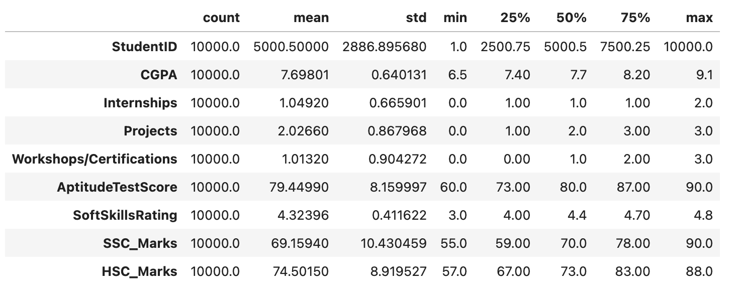
df.describe() 函式以統計方式表示 DataFrame df。為每個數值列提供了關鍵統計資訊,例如計數、均值、標準差、最小值和最大值,以初步瞭解資料分佈和主要模式。
df.describe().T
輸出
此程式碼將產生以下結果 -
探索性資料分析 (EDA)
EDA 是一種使用視覺化的資料分析技術。它用於識別趨勢和模式,以及使用統計報告和圖形表示來確認結論。在對該資料集執行 EDA 時,我們將嘗試找出獨立特徵之間的關係,即一個特徵如何影響另一個特徵。
讓我們首先快速檢視資料框中每一列的空值。
df.isnull().sum()
輸出
此程式碼將生成以下結果 -
StudentID                    0
CGPA                         0
Internships                  0
Projects                     0
Workshops/Certifications     0
AptitudeTestScore            0
SoftSkillsRating             0
ExtracurricularActivities    0
PlacementTraining            0
SSC_Marks                    0
HSC_Marks                    0
PlacementStatus              0
dtype: int64
由於資料集中沒有空值,因此我們可以繼續進行資料探索。
目標類分佈
temporary = df['PlacementStatus'].value_counts()

plt.pie(temporary.values, labels=temporary.index.values,
	shadow=True, startangle=90, autopct='%1.1f%%')
plt.title("Target Class Distributions")

plt.show()
輸出
下面的餅圖顯示了資料集的大致平衡的類分佈。雖然這可能並不完美,但它仍然是可以接受的。我們可以看到,資料集包含類別列和數字列。在我們檢視這些屬性之前,讓我們將資料集分成兩個列表。

劃分列
現在我們將把 DataFrame (df) 的列分成兩大類 - 類別列和數值列。
categorical_columns, numerical_columns = list(), list()

for col in df.columns:
   if df[col].dtype == 'object' or df[col].nunique() < 10:
      categorical_columns.append(col)
   else:
      numerical_columns.append(col)

print('Categorical Columns:', categorical_columns)
print('Numerical Columns:', numerical_columns)
輸出
此程式碼將產生以下結果 -
Categorical Columns: ['Internships', 'Projects', 'Workshops/Certifications', 'ExtracurricularActivities', 'PlacementTraining', 'PlacementStatus']
Numerical Columns: ['StudentID', 'CGPA', 'AptitudeTestScore', 'SoftSkillsRating', 'SSC_Marks', 'HSC_Marks']
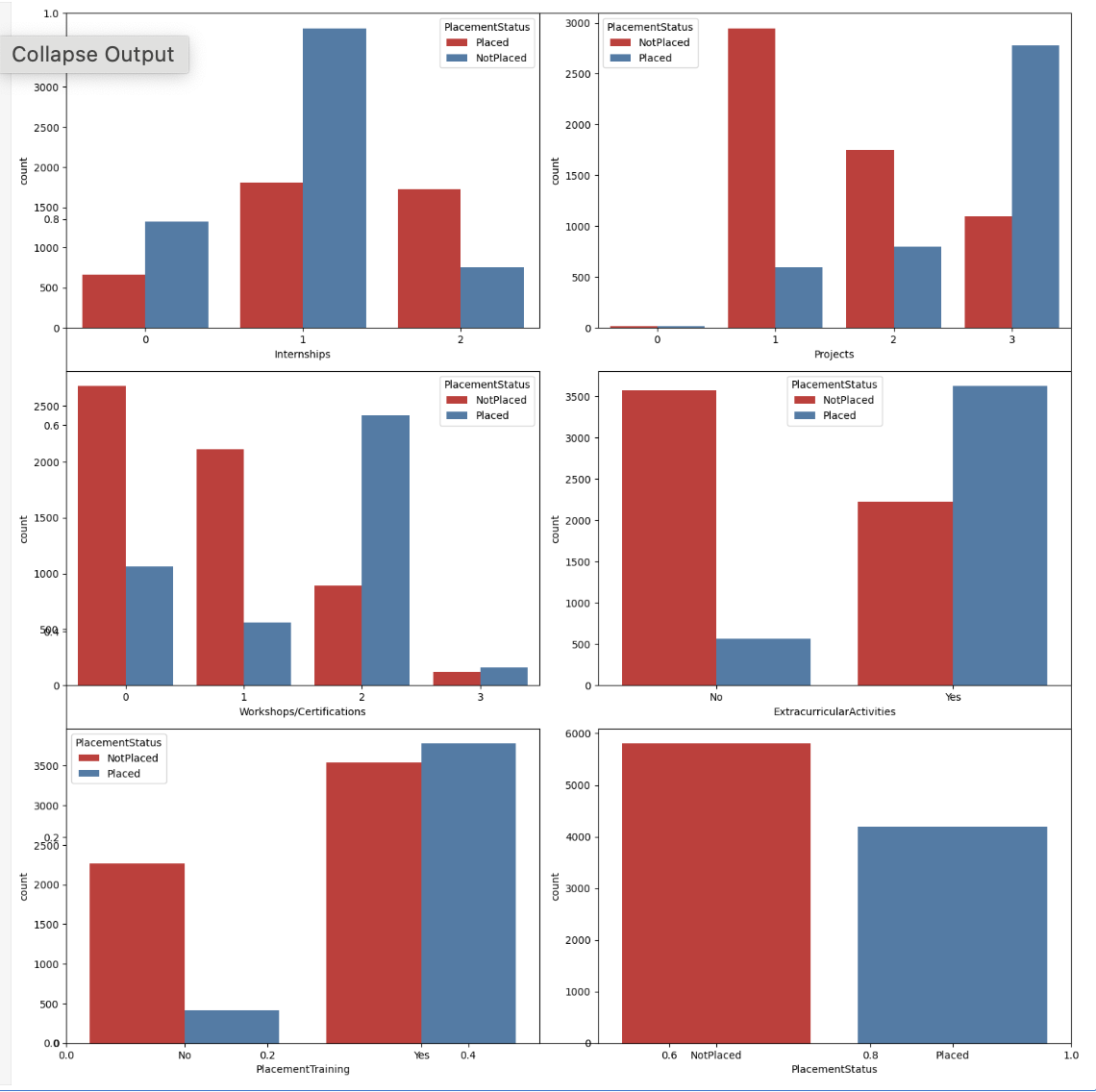
類別列的計數圖
現在,我們將使用 placement 狀態的色調,為類別列建立計數圖。
plt.subplots(figsize=(15, 15))

for i, col in enumerate(categorical_columns):
   plt.subplot(3, 2, i+1)
   sb.countplot(data=df, x=col, hue='PlacementStatus', palette='Set1')
plt.tight_layout()
plt.show()
輸出
下面提供的圖表顯示了多個模式,這些模式支援以下觀點:專注於技能發展肯定會對你的就業有所幫助。雖然確實有一些學生完成了培訓課程和專案但仍然沒有找到工作,但與那些什麼也沒做的人相比,這些人數量相對較少。
類別列的標籤編碼
在對資料集的類別特徵進行編碼後,我們將建立一個熱力圖,這將有助於識別特徵空間中與目標列高度相關的特徵。
for col in ['ExtracurricularActivities', 'PlacementTraining']:
   df[col] = df[col].map({'No':0,'Yes':1})

df['PlacementStatus']=df['PlacementStatus'].map({'NotPlaced':0, 'Placed':1})
混淆矩陣
現在我們將為上述資料集建立混淆矩陣。
sb.heatmap(df.corr(), fmt='.1f', cbar=True, annot=True, cmap='coolwarm')
plt.show()
輸出
以下結果表明沒有資料洩漏,因為資料集不包含任何高度關聯或相關的特徵。

訓練和驗證資料分割
讓我們以 85:15 的比例劃分資料集,以便在訓練期間找出模型的效能。這使我們能夠使用驗證分割的未見過的資料集來評估模型的效能。
features = df.drop(['StudentID', 'PlacementStatus'], axis=1)
target = df['PlacementStatus']

X_train, X_val, Y_train, Y_val = train_test_split(
   features,
   target,
   random_state=2023,
   test_size=0.15)

X_train.shape, X_val.shape
輸出
這將帶來以下結果 -
((8500, 10), (1500, 10))
特徵縮放
此程式碼將 StandardScaler 擬合到訓練資料以計算均值和標準差,從而在兩個資料集之間提供一致的縮放。之後,它使用這些計算出的值來轉換訓練和驗證資料。
scaler = StandardScaler()
scaler.fit(X_train)
X_train = scaler.transform(X_train)
X_val = scaler.transform(X_val)
構建和訓練模型
現在,我們可以開始使用可用的訓練資料訓練模型。由於目標列 Y_train 和 Y_val 中只有兩個可能的值,因此在這種情況下正在執行二元分類。無論模型是在訓練用於二元分類任務還是多類分類任務,都不需要單獨的規範。
ourmodel = CatBoostClassifier(verbose=100,
	iterations=1000,
	loss_function='Logloss',
	early_stopping_rounds=50,
	custom_metric=['AUC'])

ourmodel.fit(X_train, Y_train,
	eval_set=(X_val, Y_val))

y_train = ourmodel.predict(X_train)
y_val = ourmodel.predict(X_val)
輸出
這將導致以下結果 -
Learning rate set to 0.053762
0:	learn: 0.6621705	test: 0.6623146	best: 0.6623146 (0)	total: 64.3ms	remaining: 1m 4s
100:	learn: 0.3975289	test: 0.4332971	best: 0.4332174 (92)	total: 230ms	remaining: 2.05s
Stopped by overfitting detector  (50 iterations wait)

bestTest = 0.4330066724
bestIteration = 125

Shrink model to first 126 iterations.
評估模型的效能
現在讓我們使用 ROC AUC 衡量標準來評估模型在訓練和驗證資料集上的效能。
print("Training ROC AUC: ", ras(Y_train, y_train))
print("Validation ROC AUC: ", ras(Y_val, y_val))
輸出
這將帶來以下結果 -
Training ROC AUC:  0.8175316989019953
Validation ROC AUC:  0.7859439713002392