
 資料結構
資料結構 網路
網路 關係型資料庫管理系統
 作業系統
作業系統 Java
Java iOS
iOS HTML
HTML CSS
CSS Android
 Python
 C 程式設計
 C++
C++ C#
C# MongoDB
 MySQL
MySQL Javascript
 PHP
PHPPython 中的直方圖繪製和拉伸
直方圖繪製和拉伸是資料視覺化和縮放中一個強大的工具,它允許您表示數值變數的分佈,並在直方圖的資料集中將其擴充套件到值的完整範圍內。此過程可用於改善影像的對比度或提高直方圖中資料的可見性。
直方圖是資料集頻率分佈的圖形表示。它可以視覺化一組連續資料機率的潛在分佈。在本文中,我們將討論如何使用內建函式以及不使用內建函式在 Python 中建立和拉伸直方圖。
Python 中的直方圖繪製和拉伸(使用內建函式)
按照以下步驟使用 matplotlib 和 OpenCV 的內建函式繪製和拉伸直方圖,它還顯示了 RGB 通道 -
首先使用 cv2.imread 函式載入輸入影像
使用 cv2.split 函式將通道拆分為紅色、綠色和藍色
然後使用 matplotlib 庫中的 plt.hist 函式為每個通道繪製直方圖。
使用 cv2.equalizeHist 函式拉伸每個通道的對比度。
使用 cv2.merge 函式將通道合併回一起。
使用 plt.imshow 函式和 matplotlib 庫中的子圖函式並排顯示原始影像和拉伸影像。
注意 - 拉伸影像的對比度可能會導致其整體外觀發生變化,因此在評估結果時必須小心,以確保它們滿足預期的目標。
下面是 Python 中直方圖繪製和拉伸的示例程式。在此程式中,我們將假設輸入影像具有 RGB 通道。如果影像具有不同的顏色空間,則可能需要其他步驟來正確處理顏色通道。
示例
import cv2
import numpy as np
import matplotlib.pyplot as pltt
# Load the input image with RGB channels
img_sam = cv2.imread('sample.jpg', cv2.IMREAD_COLOR)
# Split the channels into red, green, and blue
rd, gn, bl = cv2.split(img_sam)
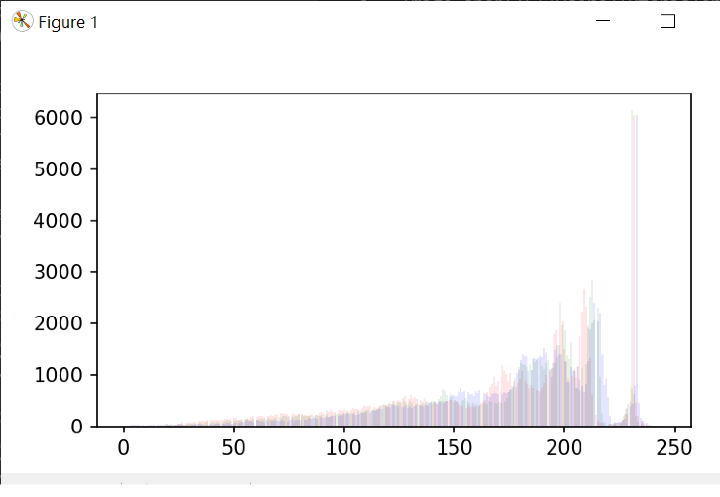
# Plot the histograms for each channel
pltt.hist(rd.ravel(), bins=277, color='red', alpha=0.10)
pltt.hist(gn.ravel(), bins=277, color='green', alpha=0.10)
pltt.hist(bl.ravel(), bins=277, color='blue', alpha=0.10)
pltt.show()
# Stretch the contrast for each channel
red_c_stretch = cv2.equalizeHist(rd)
green_c_stretch = cv2.equalizeHist(gn)
blue_c_stretch = cv2.equalizeHist(bl)
# Merge the channels back together
img_stretch = cv2.merge((red_c_stretch, green_c_stretch, blue_c_stretch))
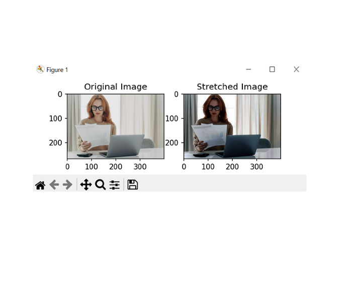
# Display the original and stretched images side by side
pltt.subplot(121)
pltt.imshow(cv2.cvtColor(img_sam, cv2.COLOR_BGR2RGB))
pltt.title('Original_Image')
pltt.subplot(122)
pltt.imshow(cv2.cvtColor(img_stretch, cv2.COLOR_BGR2RGB))
pltt.title('Stretched_Image')
pltt.show()
輸出
Python 中的直方圖繪製和拉伸(不使用內建函式)
按照以下步驟在 Python 中使用 RGB 通道進行直方圖繪製和拉伸,而無需使用內建函式。
使用 cv2.imread 函式載入輸入影像。
使用陣列切片將通道拆分為紅色、綠色和藍色。
使用巢狀迴圈和 np.zeros 函式初始化一個值為零的陣列來計算每個通道的直方圖。
透過查詢每個通道中的最小值和最大值並將畫素值線性變換到 0-255 的完整範圍內來拉伸每個通道的對比度。
對於上述步驟,使用巢狀迴圈和 np.uint8 資料型別以確保畫素值保持在 0-255 的範圍內。
使用 cv2.merge 函式將通道合併回一起。
使用 plt.imshow 函式和 matplotlib 庫中的子圖函式並排顯示原始影像和拉伸影像。
以下是執行相同操作的程式示例 -
注意 - 下面的程式假設輸入影像具有 RGB 通道,並且畫素值表示為 8 位整數。如果影像具有不同的顏色空間或資料型別,則可能需要其他步驟來正確評估結果。
示例
import cv2
import numpy as np
import matplotlib.pyplot as pltt
# Load the input image
img = cv2.imread('sample2.jpg', cv2.IMREAD_COLOR)
# Split the image into color channels
r, g, b = img[:,:,0], img[:,:,1], img[:,:,2]
# Plot the histograms for each channel
hist_r = np.zeros(256)
hist_g = np.zeros(256)
hist_b = np.zeros(256)
for i in range(img.shape[0]):
for j in range(img.shape[1]):
hist_r[r[i,j]] += 1
hist_g[g[i,j]] += 1
hist_b[b[i,j]] += 1
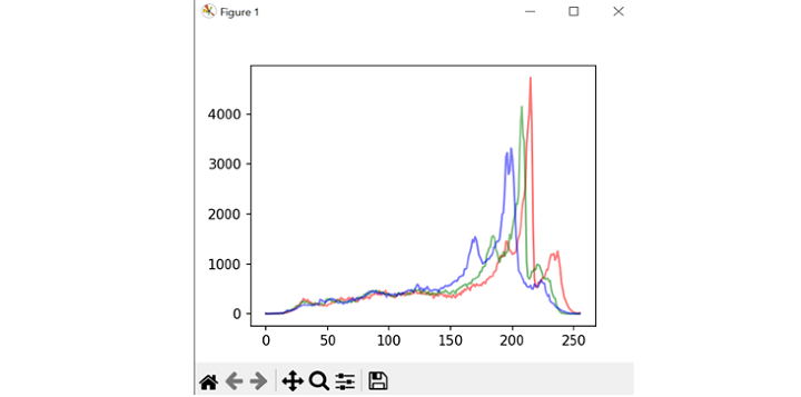
pltt.plot(hist_r, color='red', alpha=0.10)
pltt.plot(hist_g, color='green', alpha=0.10)
pltt.plot(hist_b, color='blue', alpha=0.10)
pltt.show()
# Stretch the contrast for each channel
min_r, max_r = np.min(r), np.max(r)
min_g, max_g = np.min(g), np.max(g)
min_b, max_b = np.min(b), np.max(b)
re_stretch = np.zeros((img.shape[0], img.shape[1]), dtype=np.uint8)
gr_stretch = np.zeros((img.shape[0], img.shape[1]), dtype=np.uint8)
bl_stretch = np.zeros((img.shape[0], img.shape[1]), dtype=np.uint8)
for i in range(img.shape[0]):
for j in range(img.shape[1]):
re_stretch[i,j] = int((r[i,j] - min_r) * 255 / (max_r - min_r))
gr_stretch[i,j] = int((g[i,j] - min_g) * 255 / (max_g - min_g))
bl_stretch[i,j] = int((b[i,j] - min_b) * 255 / (max_b - min_b))
# Merge the channels back together
img_stretch = cv2.merge((re_stretch, gr_stretch, bl_stretch))
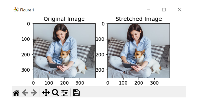
# Display the original and stretched images side by side
pltt.subplot(121)
pltt.imshow(cv2.cvtColor(img, cv2.COLOR_BGR2RGB))
pltt.title('Original Image')
pltt.subplot(122)
pltt.imshow(cv2.cvtColor(img_stretch, cv2.COLOR_BGR2RGB))
pltt.title('Stretched Image')
pltt.show()
輸出
結論
總之,Python 中的直方圖繪製和拉伸是改善數字影像對比度的一種非常有用的方法。透過繪製直方圖顏色通道,我們可以視覺化畫素值的分佈並識別低對比度區域。我們瞭解到,透過使用線性變換拉伸對比度,我們甚至可以增加影像的動態範圍並突出可能隱藏的細節。

789 次檢視
