如何使用 TensorFlow 實現邏輯迴歸？

TensorFlow 是 Google 提供的一個機器學習框架。它是一個開源框架，與 Python 結合使用以實現演算法、深度學習應用程式等等。它用於研究和生產目的。它具有最佳化技術，有助於快速執行復雜的數學運算。這是因為它使用了 NumPy 和多維陣列。

多維陣列也稱為“張量”。該框架支援使用深度神經網路。它具有高度可擴充套件性，並附帶許多流行的資料集。它使用 GPU 計算並自動管理資源。

可以使用以下程式碼行在 Windows 上安裝“tensorflow”包：

pip install tensorflow

張量是 TensorFlow 中使用的一種資料結構。它有助於連線資料流圖中的邊。此資料流圖稱為“資料流圖”。張量只不過是多維陣列或列表。

MNIST 資料集包含手寫數字，其中 60000 個用於訓練模型，10000 個用於測試訓練後的模型。這些數字已進行大小歸一化和居中處理，以適應固定大小的影像。

以下是一個示例：

示例

from __future__ import absolute_import, division, print_function
import tensorflow as tf
import numpy as np
num_classes = 10
num_features = 784
learning_rate = 0.01
training_steps = 1000
batch_size = 256
display_step = 50
from tensorflow.keras.datasets import mnist
(x_train, y_train), (x_test, y_test) = mnist.load_data()
x_train, x_test = np.array(x_train, np.float32), np.array(x_test, np.float32)
x_train, x_test = x_train.reshape([-1, num_features]), x_test.reshape([−1, num_features])
x_train, x_test = x_train / 255., x_test / 255.
train_data = tf.data.Dataset.from_tensor_slices((x_train, y_train))
train_data = train_data.repeat().shuffle(5000).batch(batch_size).prefetch(1)
A = tf.Variable(tf.ones([num_features, num_classes]), name="weight")
b = tf.Variable(tf.zeros([num_classes]), name="bias")
def logistic_reg(x):
   return tf.nn.softmax(tf.matmul(x, A) + b)
def cross_entropy(y_pred, y_true):
   y_true = tf.one_hot(y_true, depth=num_classes)
   y_pred = tf.clip_by_value(y_pred, 1e−9, 1.)
   return tf.reduce_mean(−tf.reduce_sum(y_true * tf.math.log(y_pred),1))
def accuracy_val(y_pred, y_true):
   correct_prediction = tf.equal(tf.argmax(y_pred, 1), tf.cast(y_true, tf.int64))
   return tf.reduce_mean(tf.cast(correct_prediction, tf.float32))
   optimizer = tf.optimizers.SGD(learning_rate)
def run_optimization(x, y):
   with tf.GradientTape() as g:
      pred = logistic_reg(x)
      loss = cross_entropy(pred, y)
      gradients = g.gradient(loss, [A, b])
      optimizer.apply_gradients(zip(gradients, [A, b]))
      for step, (batch_x, batch_y) in enumerate(train_data.take(training_steps), 1):
         run_optimization(batch_x, batch_y)
         if step % display_step == 0:
            pred = logistic_regression(batch_x)
            loss = cross_entropy(pred, batch_y)
            acc = accuracy_val(pred, batch_y)
            print("step: %i, loss: %f, accuracy: %f" % (step, loss, acc))
pred = logistic_reg(x_test)
print("Test accuracy is : %f" % accuracy_val(pred, y_test))
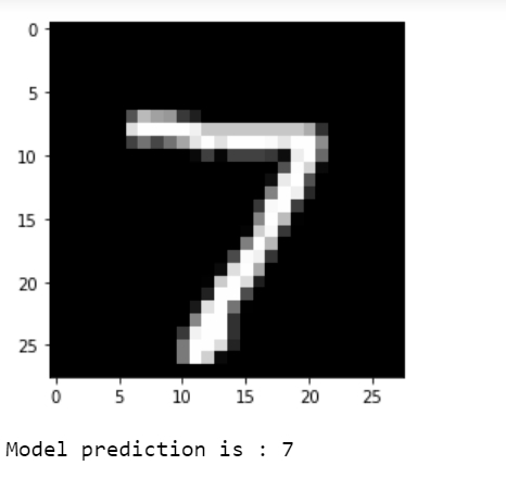
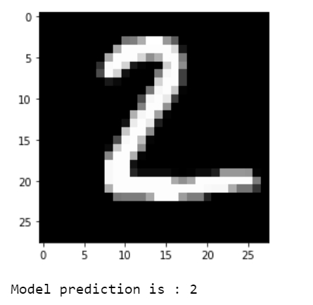
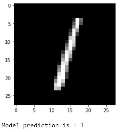
import matplotlib.pyplot as plt
n_images = 4
test_images = x_test[:n_images]
predictions = logistic_reg(test_images)
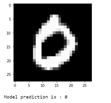
for i in range(n_images):
   plt.imshow(np.reshape(test_images[i], [28, 28]), cmap='gray')
   plt.show()
   print("Model prediction is : %i" % np.argmax(predictions.numpy()[i]))

程式碼來源 &minus https://github.com/aymericdamien/TensorFlow-Examples/blob/master/tensorflow_v2/notebooks/2_BasicModels/logistic_regression.ipynb

輸出

step: 50, loss: 2.301992, accuracy: 0.132812
step: 100, loss: 2.301754, accuracy: 0.125000
step: 150, loss: 2.303200, accuracy: 0.117188
step: 200, loss: 2.302409, accuracy: 0.117188
step: 250, loss: 2.303324, accuracy: 0.101562
step: 300, loss: 2.301391, accuracy: 0.113281
step: 350, loss: 2.299984, accuracy: 0.140625
step: 400, loss: 2.303896, accuracy: 0.093750
step: 450, loss: 2.303662, accuracy: 0.093750
step: 500, loss: 2.297976, accuracy: 0.148438
step: 550, loss: 2.300465, accuracy: 0.121094
step: 600, loss: 2.299437, accuracy: 0.140625
step: 650, loss: 2.299458, accuracy: 0.128906
step: 700, loss: 2.302172, accuracy: 0.117188
step: 750, loss: 2.306451, accuracy: 0.101562
step: 800, loss: 2.303451, accuracy: 0.109375
step: 850, loss: 2.303128, accuracy: 0.132812
step: 900, loss: 2.307874, accuracy: 0.089844
step: 950, loss: 2.309694, accuracy: 0.082031
step: 1000, loss: 2.302263, accuracy: 0.097656
Test accuracy is : 0.869700