SVM中的分離平面

---

支援向量機 (SVM) 是一種廣泛應用於手寫識別、情感分析等領域的監督學習演算法。為了分離不同的類別，SVM 計算最優超平面，該超平面或多或少準確地在兩個類別之間建立了一個邊界。

以下是一些在 SVM 中分離超平面的方法。

• 資料預處理 - SVM 需要經過標準化、縮放和中心化處理的資料，因為它們對這些特徵敏感。

• 選擇核函式 - 核函式用於將輸入轉換為更高維的空間。其中一些包括線性核、多項式核和徑向基函式。

讓我們考慮 SVM 超平面可以區分的兩種情況。

• 線性可分情況。

• 非線性可分情況。

示例 1

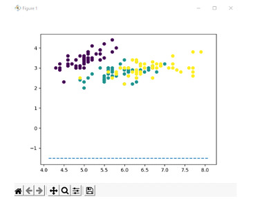
對於線性可分情況，讓我們考慮具有二維特徵的鳶尾花資料集。線性可分情況是指特徵可以透過超平面線性分離。鳶尾花資料集是展示線性可分超平面的一個很好的初學者友好方法。目標是顯示一個本質上是線性的超平面。

演算法

• 匯入所有庫

• 載入鳶尾花資料集，並將資料和目標特徵分別分配給變數 x 和 y。

• 使用 train_test_split 函式，為 x_train、x_test、y_train 和 y_test 分配值。

• 使用線性核構建 SVM 模型，並根據訓練資料點擬合模型。

• 預測標籤並列印模型的準確率。

• 使用模型將模型的權重和偏置分別作為模型的係數和直線的截距。

• 使用權重和偏置計算斜率和 y 截距。

• 在圖表中繪製資料點並展示它。

from sklearn import datasets
from sklearn.svm import SVC
from sklearn.model_selection import train_test_split as tts
from sklearn.metrics import accuracy_score
import matplotlib.pyplot as plt
import numpy as np

iris=datasets.load_iris()
x=iris.data
y=iris.target

x_train, x_test, y_train, y_test = tts(x,y,test_size=0.3,random_state=10)

#build an SVM model with linear kernel
clf=SVC(kernel='linear')

#fit the model
clf.fit(x_train,y_train)

#predict the labels
y_pred=clf.predict(x_test)

#calculate the accuracy
acc=accuracy_score(y_test,y_pred)
print("Accuracy: ", acc)

#get the hyperplane parameters
w=clf.coef_[0]
b=clf.intercept_[0]

#calculate the slope and intercept
slope = -w[0]/w[1]
y_int = -b/w[1]

#plot the dataset and hyperplane
plt.scatter(x[:,0], x[:,1], c=y)
axes=plt.gca()
x_vals=np.array(axes.get_xlim())
y_vals=y_int+slope*x_vals
plt.plot(x_vals, y_vals, '--')
plt.show()

我們將資料集分成訓練集和測試集，其中測試集佔總資料的 30%。然後，我們建立一個具有線性核的 SVM 分類器，並將模型擬合到訓練資料。

我們預測測試資料的標籤，並將獲得的結果儲存在單獨的變數中，透過將預測值與真實值進行比較來計算模型的準確率，並列印獲得的準確率，即 1.0。

然後從訓練資料集檢索超平面的引數，並計算超平面的斜率和截距，然後使用散點圖繪製，每個類別使用不同的顏色。

Accuracy: 1.0

輸出

示例 2

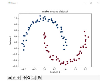
考慮一個案例不線性可分的情況。在這種情況下，我們使用 scikit-learn 庫中提供的 make_moons 資料集。make_moons 資料集是展示 2 個或多個類別不線性可分情況的好方法。因此，此示例用於描述非線性可分情況。

讓我們首先列印資料集的資料點，以便了解我們正在處理什麼。

演算法

• 匯入所有必要的庫。

• 使用 100 個樣本生成 make_moons 資料集，並具有最小的噪聲水平。

• 在圖表中繪製這些資料點並列印，並將顏色圖設定為紅色和藍色。

import matplotlib.pyplot as plt
from sklearn.datasets import make_moons

# Generate the make_moons dataset with 100 samples and a noise level of 0.05
X, y = make_moons(n_samples=100, noise=0.05, random_state=42)

# To show the dataset
plt.scatter(X[:, 0], X[:, 1], c=y, cmap=plt.cm.RdBu_r)

# Set the plot labels and title
plt.xlabel('Feature 1')
plt.ylabel('Feature 2')
plt.title('make_moons dataset')

# Show the plot
plt.show()

輸出

演算法

• 匯入程式中使用的所有庫

• 從 make_moons 資料集中生成 100 個數據樣本，噪聲儘可能低。

• 使用徑向基函式 (RBF) 核初始化 SVC 分類器，並根據分類器訓練資料點。

• 根據資料點，將前面初始化的分類器擬合到資料集。

• 查詢資料中特徵和標籤的最大值和最小值。

• 使用上述值，使用 linspace 函式構造網格。

• 要返回網格的一維表示，應用 ravel 函式並使用 np.c_ 沿第二軸切片。

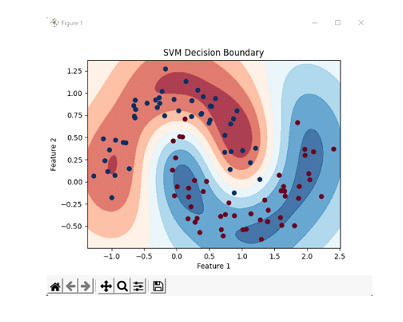
• 要定義決策邊界，建立決策邊界的等高線圖。

• 列印影像和標籤。

示例

import numpy as np
import matplotlib.pyplot as plt
from sklearn import datasets
from sklearn.svm import SVC

# load moons dataset
x, y = datasets.make_moons(n_samples=100, noise=0.15, random_state=42)

# create an SVM classifier implementing RBF kernel
clf = SVC(kernel='rbf', gamma=2)

# train the classifier on the dataset
clf.fit(X, y)

# create a meshgrid representing features and labels
x_min, x_max = x[:, 0].min() - 0.1, x[:, 0].max() + 0.1
y_min, y_max = x[:, 1].min() - 0.1, x[:, 1].max() + 0.1
xx, yy = np.meshgrid(np.linspace(x_min, x_max, 500), np.linspace(y_min, y_max, 500))
z = clf.decision_function(np.c_[xx.ravel(), yy.ravel()])
z = z.reshape(xx.shape)

# create a contour plot of the decision boundary
plt.contourf(xx, yy, z, cmap=plt.cm.RdBu, alpha=0.8)
plt.scatter(x[:, 0], x[:, 1], c=y, cmap=plt.cm.RdBu_r)

# set the plot labels and title
plt.xlabel('Feature 1')
plt.ylabel('Feature 2')
plt.title('SVM Decision Boundary')

# show the plot
plt.show()

我們透過建立 100 個樣本（噪聲級別為 0.15，隨機種子為 42）生成資料集，並建立一個 SVM 分類器，並在資料集上訓練分類器。然後，我們定義一組點來表示特徵和標籤。然後，我們計算這些點的決策函式值，並將其重新整形以匹配網格的維度。然後，我們建立決策邊界的等高線圖，其中決策函式值決定區域的顏色。我們還繪製原始資料點，不同顏色代表不同類別。

輸出

結論

支援向量機是更廣泛使用的演算法之一，用於各種領域，主要是文字和語音分類，或 NLP 中的情感分析。它在分類方面的多功能性使其成為更受歡迎的演算法之一。

在其他情況下，它有其自身的缺點。有時，SVM 在計算上可能非常密集，並且由於模型的敏感性，需要仔細檢查提供給模型的資料。