
 資料結構
資料結構 網路
網路 關係資料庫管理系統
 作業系統
作業系統 Java
Java iOS
iOS HTML
HTML CSS
CSS Android
 Python
 C 程式設計
 C++
C++ C#
C# MongoDB
 MySQL
MySQL Javascript
 PHP
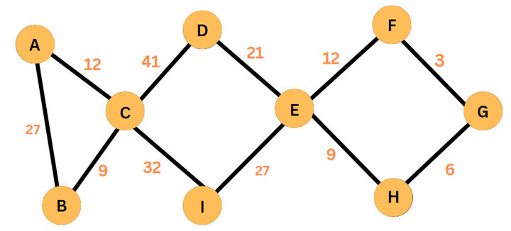
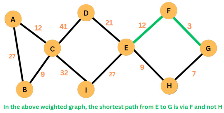
PHP有向加權圖中從源到目的地的單調最短路徑
尋路演算法基於圖搜尋技術,研究節點之間的路徑,從一個節點開始,透過連線逐步前進,直到達到目標。在這篇文章中,我們將討論加權圖以及如何在有向加權圖中計算從源節點到目標節點的單調最短路徑。
什麼是加權圖?
加權圖將圖與權重函式結合起來。也就是說,它為每條邊分配一個整數權重。
圖的邊權重有多種用途:
網路連線延遲
道路網路距離
社交網路互動的強度
有兩種主要計算方法來表示權重:
在鄰接表中,為每個頂點註冊邊權重。
維護一個單獨的集合資料結構,將每條邊對映到其權重。
單調最短路徑
如果路徑上每條邊的權重都嚴格遞增或嚴格遞減,則該路徑是單調的。
最短路徑的屬性是什麼?
最短路徑的屬性如下:
權重並不總是距離。幾何直覺很有幫助,但邊權重表示時間或成本。
最短路徑總是最簡單的。
負權重使事情變得複雜。目前,我們假設邊權重為正(或零)。
路徑是定義好的。最短路徑必須保持邊的方向。
並非所有頂點都必須可訪問。如果一個節點無法從另一個節點訪問,則不存在路徑。因此,從 s 到 t 不存在最短路徑。
在單個頂點或節點與其他節點之間,可能存在多條具有最小權重的路徑。
可以存在平行邊和自環。
迪傑斯特拉最短路徑演算法
此方法首先確定起始節點與所有直接連線節點之間最低權重的關係。它跟蹤每個權重並轉到“最接近”的節點。然後它重複計算,但這次是從原始節點開始的累積和。此過程保持這種方式,評估所有增量權重,並且始終採用到目標節點的權重最小的累積路徑。
所有節點對最短路徑 (APSP) 演算法
這將找到連線任意兩個節點的最小距離路徑。它比對網路的每兩個頂點實現 SSSP 方法更快。
APSP 透過維護已確定權重的計數來改進流程,從而同時執行多個頂點。這些確定的權重用於查詢未知頂點的最短路徑。
何時可以使用所有節點對最短路徑?
當最短路徑受阻或次優時,通常使用“所有節點對最短路徑”來探索替代方向。例如,此方法確保邏輯路由規劃中多樣化路由的最佳多條路徑。在評估所有節點之間所有或大多數替代路徑時,使用 APSP。
單源最短路徑 (SSSP)
“SSSP 演算法”在主節點和網路中的每個節點之間找到“最短加權路徑”。
它是如何工作的?
它按此順序工作:
這一切都從根節點開始,從中評估每條路徑。
選擇與根節點之間權重最小的連結並將其合併到樹中,以及其關聯的節點。
以類似的方式選擇從根節點到每個未訪問節點的下一個具有最小累積權重的關係,並將其放入樹中。
一旦沒有更多節點可以放置,則過程完成,並且獲得 SSSP。
何時可以使用此演算法?
當需要確定從已識別的初始位置到所有其他節點的最佳路徑時,使用 SSSP 演算法。由於路徑由從根開始的總路徑權重確定,因此它有利於確定到每個節點的最佳路徑,但在必須一次訪問所有節點時並不總是必要。
有向加權圖中從源到目的地的單調最短路徑
按照以下說明解決問題:
對遞增和遞減路徑分別執行兩次迪傑斯特拉演算法。
使用“迪傑斯特拉演算法求遞減最短路徑”更新從一個節點到另一個節點的最短路徑,如果節點之間的邊權重小於朝向源節點的最小距離路徑的邊權重。
對於遞增最短路徑也是如此:僅當邊長於朝向源節點的最小距離路徑的邊時,才更新從一個節點到另一個節點的最短路徑。
如果尚未到達目標頂點,則不存在合法最短路徑。
如果遞增和遞減最短路徑的兩次迪傑斯特拉演算法傳遞均未提供可行的路徑,則返回 -1。
示例
#include <bits/stdc++.h>
#include <limits>
#include <queue>
#include <vector>

using namespace std;

// Represents a vertex in the graph
class Vertex {
   public:
      int id;
      vector<int> adj_list;
      vector<double> adj_weights;

   // A constructor which accepts the id of the vertex
   Vertex(int num)
   : id(num){
   }
};

// Finds the monotonic shortest path using Dijkstra's algorithm
double shortest_path(vector<Vertex>& vertices, int src, int destination){
   int N = vertices.size() - 1;

   // Stores distance from src and edge on the shortest path from src
   vector<double> distTo(N + 1, numeric_limits<double>::max());
   vector<double> edgeTo(N + 1, numeric_limits<double>::max());

   // Setting initial distance from src to the highest value
   for (int i = 1; i <= N; i++) {
      distTo[i] = numeric_limits<double>::max();
   }

   // Monotonic decreasing pass of Dijkstra's
   distTo[src] = 0.0;
   edgeTo[src] = numeric_limits<double>::max();

   priority_queue<pair<double, int>,
   vector<pair<double, int> >,
   greater<pair<double, int> > >
   pq;
   pq.push(make_pair(0.0, src));

   while (!pq.empty()) {
      // Take the vertex with the closest current distance from src
      pair<double, int> top = pq.top();
      pq.pop();
      int closest = top.second;

      for (int i = 0; i < vertices[closest].adj_list.size(); i++) {
         int neighbor = vertices[closest].adj_list[i];
         double weight = vertices[closest].adj_weights[i];

         // Checks if the edges are decreasing and whether the current directed edge will create a shorter path
         if (weight < edgeTo[closest] && distTo[closest] + weight < distTo[neighbor]) {
            edgeTo[neighbor] = weight;
            distTo[neighbor] = distTo[closest] + weight;
            pq.push(make_pair(distTo[neighbor], neighbor));
         }
      }
   }

   // Store the result of the first pass of Dijkstra's
   double first_pass = distTo[destination];

   // Monotonic increasing pass of Dijkstra's
   for (int i = 1; i <= N; i++) {
      distTo[i] = numeric_limits<double>::max();
   }

   distTo[src] = 0.0;
   edgeTo[src] = 0.0;

   pq.push(make_pair(0.0, src));

   while (!pq.empty()) {
      // Take the vertex with the closest current distance from src
      pair<double, int> top = pq.top();
      pq.pop();
      int closest = top.second;

      for (int i = 0; i < vertices[closest].adj_list.size(); i++) {
         int neighbor = vertices[closest].adj_list[i];
         double weight = vertices[closest].adj_weights[i];

         // Checks if the edges are increasing and whether the current directed edge will create a shorter path
         if (weight > edgeTo[closest] && distTo[closest] + weight < distTo[neighbor]) {
            edgeTo[neighbor] = weight;
            distTo[neighbor] = distTo[closest] + weight;
            pq.push(make_pair(distTo[neighbor], neighbor));
         }
      }
   }

   // Store the result of the second pass of Dijkstras
   double second_pass = distTo[destination];

   if (first_pass == DBL_MAX && second_pass == DBL_MAX)
      return -1;

   return min(first_pass, second_pass);
}

// Driver Code
int main(){
   int N = 6, M = 9, src, target;

   // Create N vertices, numbered 1 to N
   vector<Vertex> vertices(N + 1, Vertex(0));

   for (int i = 1; i <= N; i++) {
      vertices[i] = Vertex(i);
   }

   // Add M edges to the graph
   vertices[1].adj_list.push_back(3);
   vertices[1].adj_weights.push_back(1.1);

   vertices[1].adj_list.push_back(5);
   vertices[1].adj_weights.push_back(2.0);

   vertices[1].adj_list.push_back(6);
   vertices[1].adj_weights.push_back(3.3);

   vertices[2].adj_list.push_back(5);
   vertices[2].adj_weights.push_back(2.7);

   vertices[3].adj_list.push_back(4);
   vertices[3].adj_weights.push_back(2.0);

   vertices[3].adj_list.push_back(5);
   vertices[3].adj_weights.push_back(1.1);

   vertices[4].adj_list.push_back(2);
   vertices[4].adj_weights.push_back(2.3);

   vertices[5].adj_list.push_back(6);
   vertices[5].adj_weights.push_back(2.4);

   vertices[6].adj_list.push_back(2);
   vertices[6].adj_weights.push_back(3.0);

   // src and destination vertices
   src = 1;
   target = 2;
   double shortest = shortest_path(vertices, src, target);
   cout << shortest << endl;
   return 0;
}
輸出
根據以上程式碼:
5.4
在加權圖中查詢最短路徑的替代方法
“貝爾曼-福特演算法”表示一種“單源最短路徑”技術。這意味著,給定一個加權網路,此方法將提供任意兩個頂點之間的最小距離路徑。
與迪傑斯特拉演算法相比,貝爾曼-福特演算法可以在具有負權重邊的圖上執行。因此,貝爾曼-福特演算法更受許多人的青睞。
此演算法的示例包括動態規劃。它從單個節點開始,然後評估可以使用一條邊訪問的更多頂點之間的距離。然後它繼續搜尋包含兩條邊的路徑,並且該過程繼續進行。貝爾曼-福特演算法採用自底向上的策略。
結論
尋路演算法可以幫助我們理解資料之間的聯絡。執行兩次迪傑斯特拉演算法可以找到源節點和目標節點之間的最小距離路徑。此方法使用邊權重來查詢一條路徑,該路徑減少了源節點和所有其他節點之間的累積權重。

490 次檢視
