
 資料結構
資料結構 網路
網路 關係型資料庫管理系統 (RDBMS)
 作業系統
作業系統 Java
Java iOS
iOS HTML
HTML CSS
CSS Android
 Python
 C語言程式設計
 C++
C++ C#
C# MongoDB
 MySQL
MySQL Javascript
 PHP
PHP如何在Pandas中使用時間序列?
時間序列資料主要用於處理隨時間變化的資料。處理這些資料在時間序列資料的分析中起著非常重要的作用。Pandas是Python中一個流行的資料操作和分析庫,它提供了強大的功能來處理時間序列資料。在本文中,我們將透過示例和解釋來了解如何在Pandas中有效地利用時間序列。
利用時間序列資料的方法
在下面的方法中,我們將使用從Kaggle獲取的Electric_production時間序列資料集。你可以從此處下載資料集。
匯入和操作時間序列資料
在Pandas中使用時間序列資料時,我們需要首先匯入必要的庫並將資料載入到DataFrame中。Pandas提供各種方法從不同的來源讀取時間序列資料,包括CSV檔案、資料庫和Web API。資料載入後,Pandas提供了強大的工具來操作、清理和預處理時間序列資料。
import pandas as pd

# Load time series data from a CSV file
data = pd.read_csv('Electric_Production.csv')

# Display the first few rows of the DataFrame
print(data.head())

# Set the 'timestamp' column as the index
data['DATE'] = pd.to_datetime(data['DATE'])
data.set_index('DATE', inplace=True)

# Resample the data to a daily frequency
daily_data = data.resample('D').mean()
輸出
       DATE  IPG2211A2N
0  1/1/1985     72.5052
1  2/1/1985     70.6720
2  3/1/1985     62.4502
3  4/1/1985     57.4714
4  5/1/1985     55.3151
時間序列資料的索引和切片
Pandas包含各種索引和切片方法,可以從時間序列資料中提取特定時間段或觀測值。Pandas中的DateTimeIndex允許基於時間進行直觀的索引和選擇。
import pandas as pd

# Load time series data from a CSV file
data = pd.read_csv('Electric_Production.csv')

# Set the 'timestamp' column as the index
data['DATE'] = pd.to_datetime(data['DATE'])
data.set_index('DATE', inplace=True)

# Resample the data to a daily frequency
daily_data = data.resample('D').mean()

# Select data for a specific date range
subset_1 = data['2017-01-01':'2017-10-30']
print(subset_1)

# Select data for a specific month
subset_2 = data[data.index.month == 3]
print(subset_2)

# Select data for a specific year
subset_3 = data[data.index.year == 2016]
print(subset_3)
輸出
            IPG2211A2N
DATE
2017-01-01    114.8505
2017-02-01     99.4901
2017-03-01    101.0396
2017-04-01     88.3530
2017-05-01     92.0805
2017-06-01    102.1532
2017-07-01    112.1538
2017-08-01    108.9312
2017-09-01     98.6154
2017-10-01     93.6137
            IPG2211A2N
DATE
1985-03-01     62.4502
1986-03-01     62.2221
1987-03-01     65.6100
1988-03-01     70.2928
1989-03-01     73.3523
1990-03-01     73.1964
1991-03-01     73.3650
1992-03-01     74.5275
1993-03-01     79.4747
1994-03-01     79.2456
1995-03-01     81.2661
1996-03-01     86.9356
1997-03-01     83.0125
1998-03-01     86.5549
1999-03-01     90.7381
2000-03-01     88.0927
2001-03-01     92.8283
2002-03-01     93.2556
2003-03-01     94.5532
2004-03-01     95.4029
2005-03-01     98.9565
2006-03-01     98.4017
2007-03-01     99.1925
2008-03-01    100.4386
2009-03-01     97.8529
2010-03-01     98.2672
2011-03-01     99.1028
2012-03-01     93.5772
2013-03-01    102.9948
2014-03-01    104.7631
2015-03-01    104.4706
2016-03-01     95.3548
2017-03-01    101.0396
            IPG2211A2N
DATE
2016-01-01    117.0837
2016-02-01    106.6688
2016-03-01     95.3548
2016-04-01     89.3254
2016-05-01     90.7369
2016-06-01    104.0375
2016-07-01    114.5397
2016-08-01    115.5159
2016-09-01    102.7637
2016-10-01     91.4867
2016-11-01     92.8900
2016-12-01    112.7694
處理缺失資料
時間序列資料通常包含缺失值,這可能會阻礙分析和建模。Pandas提供了幾種處理缺失資料的方法,例如插值、前向填充或後向填充。這些方法有助於確保時間序列的連續性。
import pandas as pd

# Load time series data from a CSV file
data = pd.read_csv('Electric_Production.csv')

# Display the first few rows of the DataFrame
# print(data.head())

# Set the 'timestamp' column as the index
data['DATE'] = pd.to_datetime(data['DATE'])
data.set_index('DATE', inplace=True)

# Resample the data to a daily frequency
daily_data = data.resample('D').mean()

## Interpolate missing values
data['value'] = data['value'].interpolate()
print(data.head())

# Forward-fill missing values
data['value'] = data['value'].ffill()
print(data.head())

# Backward-fill missing values
data['value'] = data['value'].bfill()
print(data.head())
輸出
               value
DATE
1985-01-01  72.5052
1985-02-01  70.6720
1985-03-01  64.0717
1985-04-01  57.4714
1985-05-01  55.3151
              value
DATE
1985-01-01  72.5052
1985-02-01  70.6720
1985-03-01  64.0717
1985-04-01  57.4714
1985-05-01  55.3151
              value
DATE
1985-01-01  72.5052
1985-02-01  70.6720
1985-03-01  64.0717
1985-04-01  57.4714
1985-05-01  55.3151
重取樣和頻率轉換
重取樣涉及更改時間序列資料的頻率。Pandas提供用於時間序列資料上取樣(增加頻率)和下采樣(降低頻率)的方法。這允許在不同的時間間隔內聚合或插值資料。
import pandas as pd

# Load time series data from a CSV file
data = pd.read_csv('Electric_Production.csv')

# Display the first few rows of the DataFrame
# print(data.head())

# Set the 'timestamp' column as the index
data['DATE'] = pd.to_datetime(data['DATE'])
data.set_index('DATE', inplace=True)

# Resample the data to a daily frequency
daily_data = data.resample('D').mean()
print(daily_data.head())

# Resample the data to a weekly frequency, taking the mean value
weekly_data = data.resample('W').mean()
print(weekly_data.head())

# Resample the data to a monthly frequency, taking the sum value
monthly_data = data.resample('M').sum()
print(weekly_data.head())
輸出
              value
DATE
1985-01-01  72.5052
1985-01-02      NaN
1985-01-03      NaN
1985-01-04      NaN
1985-01-05      NaN
              value
DATE
1985-01-06  72.5052
1985-01-13      NaN
1985-01-20      NaN
1985-01-27      NaN
1985-02-03  70.6720
              value
DATE
1985-01-06  72.5052
1985-01-13      NaN
1985-01-20      NaN
1985-01-27      NaN
1985-02-03  70.6720
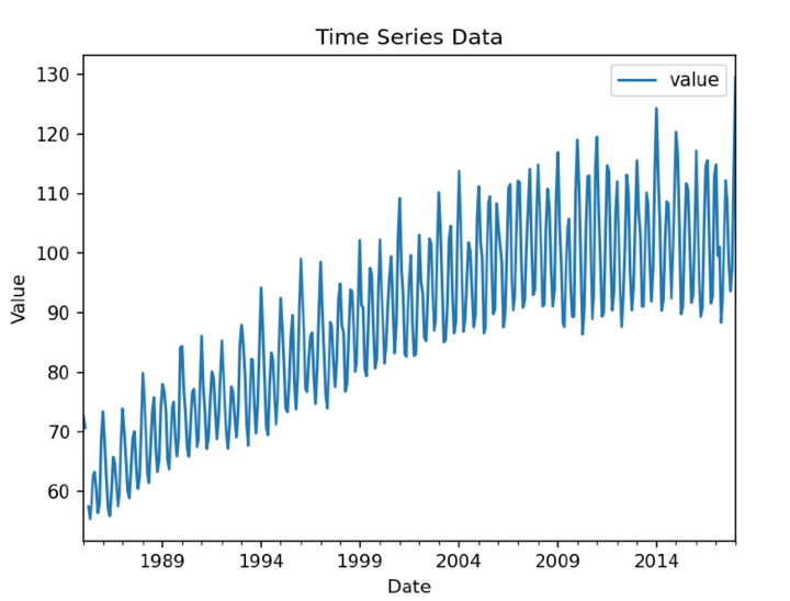
繪製和視覺化時間序列資料
Pandas與Matplotlib(一個流行的資料視覺化庫)整合,可以輕鬆建立時間序列資料的有見地的圖表和視覺化。視覺化可以幫助理解資料中的趨勢、模式和異常。
import pandas as pd
import matplotlib.pyplot as plt

# Load time series data from a CSV file
data = pd.read_csv('Electric_Production.csv')

# Display the first few rows of the DataFrame
# print(data.head())

# Set the 'timestamp' column as the index
data['DATE'] = pd.to_datetime(data['DATE'])
data.set_index('DATE', inplace=True)

# Plot the time series data
data.plot()
plt.title('Time Series Data')
plt.xlabel('Date')
plt.ylabel('Value')
plt.show()
輸出
結論
在本文中,我們討論瞭如何使用pandas的功能來使用時間序列資料。從匯入和預處理資料到高階分析和視覺化,Pandas簡化了整個時間序列分析工作流程。透過利用本文中討論的功能,分析師和資料科學家可以獲得有價值的見解,並根據基於時間的資料做出明智的決策。

96 次瀏覽
