
 資料結構
資料結構 網路
網路 關係型資料庫管理系統
 作業系統
作業系統 Java
Java iOS
iOS HTML
HTML CSS
CSS Android
 Python
 C 語言程式設計
 C++
C++ C#
C# MongoDB
 MySQL
MySQL Javascript
 PHP
PHPTensorFlow 中的 CIFAR-10 影像分類
影像分類是計算機視覺中一項基本任務,它涉及根據影像內容識別和分類影像。CIFAR-10 是一個眾所周知的包含 60,000 張 32×32 彩色影像的資料集,分為 10 個類別,每個類別包含 6,000 張影像。
TensorFlow 是一個強大的框架,它提供了各種工具和 API 用於構建和訓練機器學習模型。它廣泛用於深度學習應用,並且擁有龐大的開發者社群參與其開發。TensorFlow 提供了一個名為 Keras 的高階 API,它使構建和訓練深度神經網路變得容易。
在本教程中,我們將探討如何使用 TensorFlow(一個流行的開源機器學習框架)對 CIFAR-10 執行影像分類。
載入資料
任何機器學習專案的第一個步驟都是準備資料。在本例中,我們將使用 CIFAR-10 資料集,它可以使用 TensorFlow 的內建資料集模組輕鬆下載。
讓我們從匯入必要的模組開始 -
import tensorflow as tf
from tensorflow.keras.datasets import cifar10
接下來,我們可以使用 cifar10 模組中的 load_data() 函式載入 CIFAR-10 資料集 -
# Load the CIFAR-10 dataset
(train_images, train_labels), (test_images, test_labels) = cifar10.load_data()
此程式碼將訓練和測試影像及其相應的標籤載入到四個 NumPy 陣列中。train_images 和 test_images 陣列包含影像本身,而 train_labels 和 test_labels 陣列包含相應的標籤(即,從 0 到 9 的整數,表示 10 個類別)。
始終建議視覺化資料集中的幾個示例,以便了解我們正在處理的內容 -
import matplotlib.pyplot as plt
import numpy as np

# Define the class names for visualization purposes
class_names = ['airplane', 'automobile', 'bird', 'cat', 'deer','dog', 'frog', 'horse', 'ship', 'truck']

# Plot a few examples
plt.figure(figsize=(10,10))
for i in range(25):
   plt.subplot(5,5,i+1)
   plt.xticks([])
   plt.yticks([])
   plt.grid(False)
   plt.imshow(train_images[i], cmap=plt.cm.binary)
   plt.xlabel(class_names[train_labels[i][0]])
plt.show()
這將顯示訓練集中 25 張影像的網格,以及它們相應的標籤。
資料預處理
在我們可以使用 CIFAR-10 資料集訓練模型之前,我們需要預處理資料。我們需要採取兩個主要預處理步驟 -
規範化畫素值
影像中的畫素值範圍從 0 到 255。透過將這些值縮放到 0 到 1 的範圍內,我們可以提高模型的訓練效能 -
# Normalize the pixel values to be between 0 and 1
train_images, test_images = train_images / 255.0, test_images / 255.0
對標籤進行獨熱編碼
CIFAR-10 資料集中的標籤是從 0 到 9 的整數。但是,為了訓練模型對影像進行分類,我們需要將這些整數轉換為獨熱編碼向量。TensorFlow 提供了一個方便的函式來執行此操作 -
train_labels = tf.keras.utils.to_categorical(train_labels)
test_labels = tf.keras.utils.to_categorical(test_labels)
構建模型
現在我們已經預處理了資料,我們可以開始構建我們的模型了。我們將使用卷積神經網路 (CNN),這是一種特別適合影像分類任務的神經網路型別。
以下是我們將用於 CIFAR-10 模型的架構 -
卷積層 - 我們將從兩個卷積層開始,每個卷積層後面跟著一個最大池化層。卷積層的目的是從輸入影像中學習特徵,而最大池化層則對卷積層的輸出進行下采樣。
扁平化層 - 然後我們將卷積層的輸出扁平化為一個一維向量,該向量將傳遞給全連線層。
全連線層 - 我們將使用兩個全連線層,每個層包含 512 個神經元和一個 ReLU 啟用函式。全連線層的目的是根據卷積層學習的特徵學習類別機率。
輸出層 - 最後,我們將新增一個包含 10 個神經元的輸出層(每個類別一個),以及一個 softmax 啟用函式,它將生成最終的類別機率。
以下是構建此模型的程式碼 -
# Define the CNN model
model = tf.keras.models.Sequential([
   tf.keras.layers.Conv2D(32, (3, 3), activation='relu', input_shape=(32, 32, 3)),
   tf.keras.layers.MaxPooling2D((2, 2)),
   tf.keras.layers.Conv2D(64, (3, 3), activation='relu'),
   tf.keras.layers.MaxPooling2D((2, 2)),
   tf.keras.layers.Conv2D(64, (3, 3), activation='relu'),
   tf.keras.layers.Flatten(),
   tf.keras.layers.Dense(64, activation='relu'),
   tf.keras.layers.Dense(10, activation='softmax')
])
編譯和訓練模型
現在我們已經定義了模型,我們需要對其進行編譯並在 CIFAR-10 資料集上進行訓練。我們將使用 compile() 方法指定訓練期間使用的損失函式、最佳化器和指標 -
以下是編譯模型的程式碼 -
# Compile the model
model.compile(optimizer='adam',
   loss='categorical_crossentropy',
   metrics=['accuracy'])
我們使用 adam 最佳化器,這是一種流行的隨機梯度下降 (SGD) 變體,它在訓練期間自適應地調整學習率。我們還使用 categorical_crossentropy 損失函式,這是多類分類問題的常用選擇。最後,我們指定準確率指標,該指標將用於評估訓練期間模型的效能。
要訓練模型,我們只需呼叫 fit 方法並傳入訓練資料和標籤 -
# Train the model
history = model.fit(train_images, train_labels, epochs=10, validation_data=(test_images, test_labels))
在上面的程式碼中,我們使用訓練資料訓練模型 10 個 epoch,並在測試資料上對其進行驗證。`fit()` 方法返回一個 `History` 物件,其中包含有關訓練過程的資訊,例如每個 epoch 的損失和準確率值。
以下是包含有關訓練過程資訊的輸出 -
Epoch 1/10
1563/1563 [==============================] - 55s 34ms/step - loss: 1.7739 - accuracy: 0.3845 - val_loss: 1.4289 - val_accuracy: 0.4986
Epoch 2/10
1563/1563 [==============================] - 62s 40ms/step - loss: 1.2955 - accuracy: 0.5384 - val_loss: 1.2574 - val_accuracy: 0.5585
Epoch 3/10
1563/1563 [==============================] - 57s 36ms/step - loss: 1.1365 - accuracy: 0.6024 - val_loss: 1.1261 - val_accuracy: 0.6079
Epoch 4/10
1563/1563 [==============================] - 56s 36ms/step - loss: 1.0434 - accuracy: 0.6355 - val_loss: 1.0228 - val_accuracy: 0.6490
Epoch 5/10
1563/1563 [==============================] - 57s 36ms/step - loss: 0.9579 - accuracy: 0.6663 - val_loss: 1.0293 - val_accuracy: 0.6466
Epoch 6/10
1563/1563 [==============================] - 56s 36ms/step - loss: 0.8967 - accuracy: 0.6868 - val_loss: 1.0676 - val_accuracy: 0.6463
Epoch 7/10
1563/1563 [==============================] - 50s 32ms/step - loss: 0.8372 - accuracy: 0.7088 - val_loss: 1.0286 - val_accuracy: 0.6571
Epoch 8/10
1563/1563 [==============================] - 56s 36ms/step - loss: 0.7923 - accuracy: 0.7266 - val_loss: 1.0569 - val_accuracy: 0.6498
Epoch 9/10
1563/1563 [==============================] - 50s 32ms/step - loss: 0.7490 - accuracy: 0.7413 - val_loss: 1.0367 - val_accuracy: 0.6585
Epoch 10/10
1563/1563 [==============================] - 59s 38ms/step - loss: 0.7065 - accuracy: 0.7548 - val_loss: 1.0404 - val_accuracy: 0.6713
評估模型
訓練模型後,我們可以使用 evaluate 方法評估其在測試集上的效能 -
# Evaluate the model on the test set
test_loss, test_acc = model.evaluate(test_images, test_labels)
print('Test accuracy:', test_acc)
這將列印模型的測試準確率,這表明它在分類從未見過的影像方面的表現如何。
我們還可以使用 Matplotlib 視覺化隨時間推移的訓練和驗證準確率 -
# Plot the training and validation accuracy over time
plt.plot(history.history['accuracy'], label='accuracy')
plt.plot(history.history['val_accuracy'], label='val_accuracy')
plt.xlabel('Epoch')
plt.ylabel('Accuracy')
plt.ylim([0.5, 1])
plt.legend(loc='lower right')
plt.show()
以下是準確率曲線可能的樣子示例 -
313/313 [==============================] - 3s 8ms/step - loss: 1.0404 - accuracy: 0.6713
Test accuracy: 0.6712999939918518
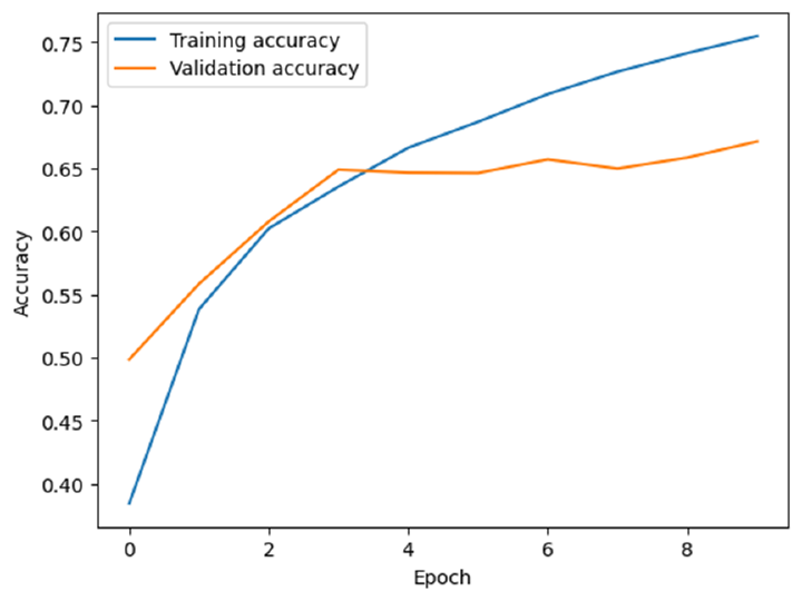
這將顯示訓練 10 個 epoch 期間訓練和驗證準確率的圖表。我們可以看到,我們的模型實現了大約 75% 的訓練準確率和大約 67% 的驗證準確率,考慮到 CIFAR-10 資料集的小尺寸,這還不錯。
做出預測
訓練和評估模型後,我們可以使用它對新影像進行預測。以下是如何進行預測的示例 -
# Load a new image
new_image = plt.imread(r'C:\Users\Leekha\Desktop\sparrow.jpg')
new_image = tf.image.resize(new_image, (32, 32))

# Reshape the image to match the input shape of the model
new_image = np.expand_dims(new_image, axis=0)

# Make a prediction
predictions = model.predict(new_image)

# Get the index of the predicted class
predicted_class_index = np.argmax(predictions)

# Map the index to the corresponding class name
predicted_class_name = class_names[predicted_class_index]

# Print the predicted class name
print('Predicted class:', predicted_class_name)
它將給出以下預測 -
1/1 [==============================] - 0s 32ms/step
Predicted class: bird
讓我們從訓練好的模型中再做一個預測 -
# Load a new image
new_image = plt.imread(r'C:\Users\Leekha\Desktop\car.jpg')
new_image = tf.image.resize(new_image, (32, 32))

# Reshape the image to match the input shape of the model
new_image = np.expand_dims(new_image, axis=0)

# Make a prediction
predictions = model.predict(new_image)

# Get the index of the predicted class
predicted_class_index = np.argmax(predictions)

# Map the index to the corresponding class name
predicted_class_name = class_names[predicted_class_index]

# Print the predicted class name
print('Predicted class:', predicted_class_name)
它將給出以下預測 -
1/1 [==============================] - 0s 19ms/step
Predicted class: automobile
在上面的程式碼塊中,我們首先使用 plt.imread 載入新影像,並將其調整大小以匹配模型的輸入形狀。然後,我們將影像的維度擴充套件以匹配模型的批次大小。
最後,我們使用模型的 predict 方法獲取影像的預測類別機率。我們使用 np.argmax 查詢預測類別的索引,然後在 class_names 列表中查詢相應的類名。然後將預測的類名列印到控制檯。
結論
在本文中,我們探討了如何使用 TensorFlow 和 Keras 對 CIFAR-10 資料集執行影像分類。我們構建了一個卷積神經網路 (CNN),並在 CIFAR-10 資料集上對其進行了訓練,實現了大約 67% 的測試準確率。我們還使用 Matplotlib 可視化了隨時間推移的訓練和驗證準確率。

428 次檢視
