
 資料結構
資料結構 網路
網路 關係型資料庫管理系統 (RDBMS)
 作業系統
作業系統 Java
Java iOS
iOS HTML
HTML CSS
CSS Android
 Python
 C語言程式設計
 C++
C++ C#
C# MongoDB
 MySQL
MySQL Javascript
 PHP
PHP使用Python進行機器學習的醫療保險價格預測
與許多其他領域一樣,預測分析在金融和保險領域也相當有用。使用這種機器學習技術,我們可以找出有關任何保險單的有用資訊,從而節省大量資金。在這裡,我們將對醫療保險資料集使用這種預測分析方法。
這裡的問題陳述是,我們擁有一些具有某些屬性的人的資料集。使用Python中的機器學習,我們必須從這個資料集中找出相關資訊,並且還必須預測一個人將不得不支付的保險價格。
演算法
步驟 1 − 匯入numpy、pandas、matplotlib、seaborn和sklearn等庫,並將資料集載入為pandas資料幀。
步驟 2 − 為了清理資料,首先檢查空值。如果發現空值,則查詢各種特徵之間的關係並估算空值。如果沒有,那麼我們就可以開始了。
步驟 3 − 現在執行EDA,這意味著檢查各種自變數之間的關係。
步驟 4 − 查詢異常值並調整它們。
步驟 5 − 繪製熱圖以找出高度相關的變數。
步驟 6 − 將資料集拆分為測試集和訓練集,並使用StandardScaler標準化資料。
步驟 7 − 現在在這個資料上訓練一些機器學習模型,並使用mape來檢查哪個模型效果最好。
示例
在這個例子中,我們將使用一個醫療保險資料集(你可以在此處找到),然後我們將執行預測一個人必須為特定醫療保險支付的保險價格所需的各種步驟。
#import the required libraries
import numpy as np
import pandas as pd
import seaborn as sb
import matplotlib.pyplot as plt
from sklearn.model_selection import train_test_split
from sklearn.preprocessing import StandardScaler, LabelEncoder
from sklearn.metrics import mean_absolute_percentage_error as mape
from sklearn.linear_model import LinearRegression, Lasso, Ridge
from xgboost import XGBRegressor
from sklearn.ensemble import RandomForestRegressor, AdaBoostRegressor
import warnings
warnings.filterwarnings('ignore')
#load and print the dataset
df = pd.read_csv('insurance_dataset.csv')
df.head()
df.shape
df.info()
df.describe()
#check for null values
df.isnull().sum()
#see the relation between independent features
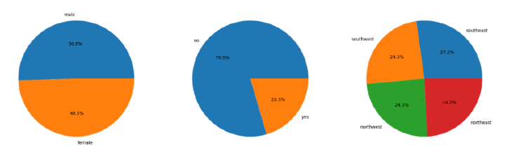
#pie charts
features = ['sex', 'smoker', 'region']
plt.subplots(figsize=(20, 10))
for i, col in enumerate(features):
plt.subplot(1, 3, i + 1)
x = df[col].value_counts()
plt.pie(x.values, labels=x.index, autopct='%1.1f%%')
plt.show()
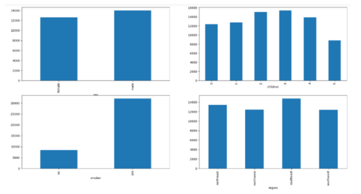
#bar graphs
features = ['sex', 'children', 'smoker', 'region']
plt.subplots(figsize=(20, 10))
for i, col in enumerate(features):
plt.subplot(2, 2, i + 1)
df.groupby(col).mean()['charges'].plot.bar()
plt.show()
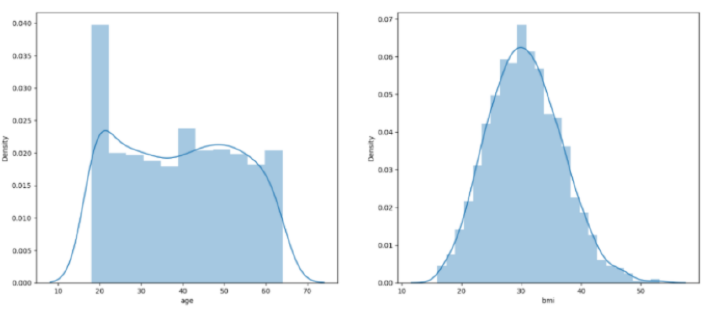
#plots
features = ['age', 'bmi']
plt.subplots(figsize=(17, 7))
for i, col in enumerate(features):
plt.subplot(1, 2, i + 1)
sb.distplot(df[col])
plt.show()
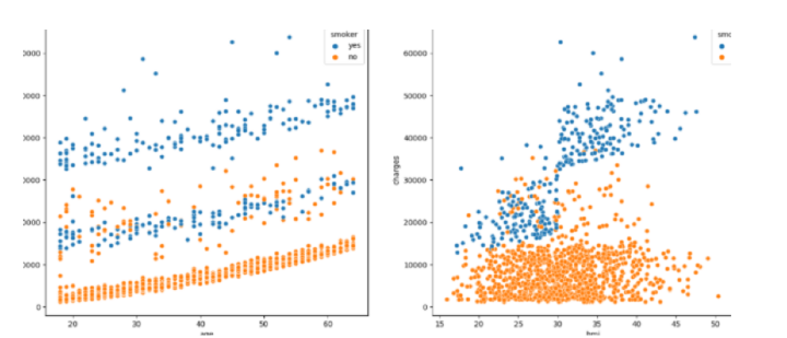
#scatterplots
features = ['age', 'bmi']
plt.subplots(figsize=(17, 7))
for i, col in enumerate(features):
plt.subplot(1, 2, i + 1)
sb.scatterplot(data=df, x=col, y='charges', hue='smoker')
plt.show()
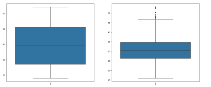
#check for outliers
features = ['age', 'bmi']
plt.subplots(figsize=(17, 7))
for i, col in enumerate(features):
plt.subplot(1, 2, i + 1)
sb.boxplot(df[col])
plt.show()
#adjust the outliers
df.shape, df[df['bmi']<45].shape
df = df[df['bmi']<50]
for col in df.columns:
if df[col].dtype == object:
le = LabelEncoder()
df[col] = le.fit_transform(df[col])
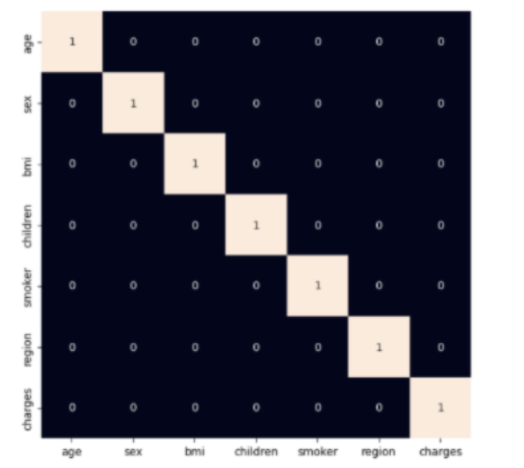
#use heatmap to see highly correlated variables
plt.figure(figsize=(7, 7))
sb.heatmap(df.corr() > 0.8, annot=True, cbar=False)
plt.show()
#split the dataset into train and test sets
features = df.drop(['charges'], axis=1)
target = df['charges']
X_train, X_val,\
Y_train, Y_val = train_test_split(features, target, test_size=0.1, random_state=22)
X_train.shape, X_val.shape
#fit the data
scaler = StandardScaler()
X_train = scaler.fit_transform(X_train)
X_val = scaler.transform(X_val)
#find the performance of various models
models = [LinearRegression(), XGBRegressor(),
RandomForestRegressor(), AdaBoostRegressor(),
Lasso(), Ridge()]
for i in range(6):
models[i].fit(X_train, Y_train)
print(f'{models[i]} : ')
pred_train = models[i].predict(X_train)
print('Training Error : ', mape(Y_train, pred_train))
pred_val = models[i].predict(X_val)
print('Validation Error : ', mape(Y_val, pred_val))
print()
匯入所需的庫後,資料集將儲存到python資料框中。然後,程式碼檢查資料集中是否存在空值,並相應地繪製餅圖和條形圖以視覺化資料集中性別、地區和吸菸者列的分佈和比例。
然後,顯示直方圖和散點圖以視覺化年齡和bmi與費用變數的分佈和關係。檢查年齡和bmi列,並透過過濾掉極值來進行修改。之後,將性別、吸菸者和地區列中的值轉換為數值形式,並建立一個熱圖以視覺化資料集中列之間的關係。
然後將資料集拆分為訓練集和驗證集。根據訓練集和驗證集上的平均絕對百分比誤差,訓練和評估各種迴歸模型。
輸出
<class 'pandas.core.frame.DataFrame'>
RangeIndex: 1338 entries, 0 to 1337
Data columns (total 7 columns):
 #   Column    Non-Null Count  Dtype
---  ------    --------------  -----
 0   age       1338 non-null   int64
 1   sex       1338 non-null   object
 2   bmi       1338 non-null   float64
 3   children  1338 non-null   int64
 4   smoker    1338 non-null   object
 5   region    1338 non-null   object
 6   charges   1338 non-null   float64
dtypes: float64(2), int64(2), object(3)
memory usage: 73.3+ KB
LinearRegression() −
Training Error :  0.42160312973300035
Validation Error :  0.36819643775368394
XGBRegressor() −
Training Error :  0.07414118093426757
Validation Error :  0.43487251393507226
RandomForestRegressor() −
Training Error :  0.11931475932482996
Validation Error :  0.33574049059141486
AdaBoostRegressor() −
Training Error :  0.6166709629183661
Validation Error :  0.5758503954769271
Lasso() −
Training Error :  0.42160217445355996
Validation Error :  0.36821456297631355
Ridge() −
Training Error :  0.42182509871430085
Validation Error :  0.3685041955294438
您可以看到XGBRegressor的MAPE(平均絕對百分比誤差)值最小。這意味著該模型預測的價格非常接近實際價格,因此可以認為是該專案的最佳模型。
結論
為了進行這種醫療保險價格預測,您還可以使用其他模型,例如K近鄰(KNN)、支援向量機(SVM)、隨機森林(RF)和樸素貝葉斯等。此外,此處的資料大多已預處理。但是,您可以根據需要自行預處理它。此外,可以以相同的方式對具有其他幾個特徵的資料集進行類似的預測。

515 次瀏覽
