機器學習中學習曲線的應用詳解

---

簡介

機器學習的核心在於教會計算機學習模式並在無需顯式程式設計的情況下做出決策。它透過支援能夠解決複雜問題的智慧系統，徹底改變了多個行業。機器學習中一個經常被忽視的關鍵方面是學習曲線。這些曲線反映了一個基本的過程，模型隨著時間的推移逐漸提高其預測能力。在本文中，我們將透過創意示例和詳細解釋來探索機器學習中學習曲線的迷人世界。

機器學習中的學習曲線

學習曲線是圖形化的表示，用於視覺化模型效能隨著資料集大小的增加或訓練過程的進行而發生的變化。通常將其描繪成將模型錯誤率（在訓練資料和測試資料上）與各種樣本大小或迭代次數進行比較的圖表，從而提供了關於模型泛化能力的有價值的見解。

富有洞察力的旅程

想象一下，踏上一段穿越未知領域的冒險之旅——在深入機器學習令人興奮的領域（錯綜複雜的演算法和方法）時，也適用了類似的比喻。

考慮使用數量不斷增加的帶標籤資料訓練影像分類演算法——最初從小規模開始，但逐漸轉向從數千張到數百萬張影像的更大資料集。在整個過程中，機器會適應識別給定資料集中存在的模式——從簡單開始，然後隨著從額外樣本中獲得更多知識而發展為更復雜的模式。

初始階段 - 高偏差（欠擬合）

當我們的虛擬影像分類器遇到其初始任務相關的挑戰時，僅使用有限數量的觀察結果（例如 100 張影像），由於高偏差或欠擬合問題，它很可能泛化能力較差。過於簡單的表示未能捕捉到更大量資料集中存在的關鍵細微差別——類似於嘗試性地瀏覽未探索的路徑，但由於資訊不足而無法得出準確的預測或分類。

中期階段 - 最佳平衡

在我們的探險中進一步前進，需要向演算法提供包含數千張（例如 10,000 張）影像的逐漸增大的帶標籤資料集。在此階段，學習者力求在捕捉內在模式和避免過度泛化或過度複雜性之間取得最佳平衡。隨著模型吸收更多知識，其學習曲線逐漸趨於平緩——顯示出一個收斂點，其中訓練誤差趨於平穩，而測試誤差逐漸減小。此階段代表了一個重要的里程碑，表明在處理新的、未見過的資料方面具有良好的泛化能力。

高階階段 - 高方差（過擬合）

冒險進入機器學習探索之旅的最深處，揭示了包含數百萬（或更多）帶標籤影像的高度多樣化資料集帶來的新挑戰。

方法 1：Python 程式碼 - 在機器學習中使用學習曲線

學習曲線是任何機器學習工具包中不可或缺的工具，可以釋放演算法效能的真正力量。

演算法

步驟 1：匯入必要的庫（scikit-learn、matplotlib）。

步驟 2：使用 scikit-learn 中的 load_digits() 函式載入數字資料集。

步驟 3：分別將特徵和標籤分配給 X 和 Y。

步驟 4：使用 scikit-learn 中的 learning_curve() 函式生成學習曲線

• 對支援向量機分類器 (SVC) 使用線性核

• 使用 10 折交叉驗證

• 使用準確率作為評分指標

• 將訓練大小從 10% 更改到 100%

步驟 5：計算每個訓練大小下各折的訓練分數和測試分數的均值和標準差。

步驟 6：繪製訓練準確率均值與訓練樣本數量的圖表，並用陰影（用於透明度）表示標準差。

步驟 7：繪製交叉驗證準確率均值與訓練樣本數量的圖表，並用陰影（用於透明度）表示標準差。

步驟 8：新增軸標籤和圖表標題，顯示圖表。

示例

#Importing the required libraries that is load_digits, learning_curve, SVC (Support Vector Classifier), matplotlib
from sklearn.datasets import load_digits
from sklearn.model_selection import learning_curve
from sklearn.svm import SVC
import matplotlib.pyplot as plt
import numpy as np

#Loading the digits dataset and storing in digits variable
digits = load_digits()
#Storing the features to the variables
X, y = digits.data, digits.target

#The learning curve is generated using the required function
train_sizes, train_scores, test_scores = learning_curve(
#linear kernel is used for SVC
    SVC(kernel='linear'), X, y,
#cv is assigned with value 10-fold cross validation
    cv=10,
#Scoring variable is assigned to hold scoring metric
    scoring='accuracy',
#Using the parallel processing
    n_jobs=-1,
#By interchanging the training size from 10% to 100%
    train_sizes=np.linspace(0.1, 1.0, 10),
)
#To get the mean of the training scores
train_mean = np.mean(train_scores, axis=1)
#To get the standard deviation of the training scores
train_std = np.std(train_scores, axis=1)
#To get the mean test scores across folds
test_mean = np.mean(test_scores, axis=1)
#To get the standard deviation test scores across folds
test_std = np.std(test_scores, axis=1)
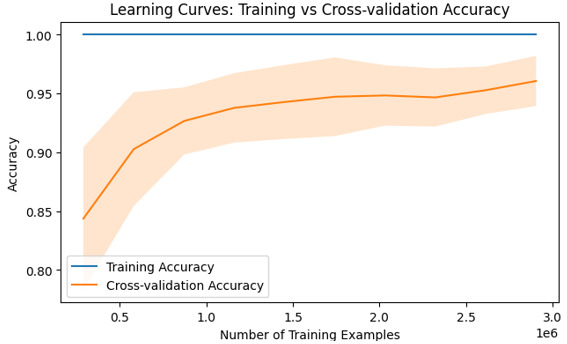
#It plots the graph between training accuracy vs number of training examples
plt.plot(train_sizes * len(y), train_mean,label="Training Accuracy")
#filling the area between mean and standard deviation with alpha 0.2
plt.fill_between(train_sizes * len(y), train_mean - train_std,
                 train_mean + train_std,alpha=0.2)
#It plots the graph between cross-validation accuracy vs number of training examples
plt.plot(train_sizes * len(y), test_mean,label="Cross-validation Accuracy")
# filling the area between mean and standard deviation with alpha 0.2
plt.fill_between(train_sizes * len(y), test_mean - test_std,
                 test_mean + test_std,alpha=0.2)
#Plotting the x axis with Number of training examples
plt.xlabel("Number of Training Examples")
#Plotting the y axis with accuracy
plt.ylabel("Accuracy")
#The plot with title “Learning curves: Training vs Cross-Validation Accuracy”
plt.title("Learning Curves: Training vs Cross-validation Accuracy")
#Adding the legends and displaying the output
plt.legend()
plt.show()

輸出

結論

理解學習曲線在機器學習中至關重要，因為它們提供了對模型效能趨勢（隨著資料集大小或複雜程度的變化）的見解。透過使用如上所示的 Python 程式碼將錯誤率與樣本大小之間的關係視覺化，研究人員可以診斷諸如過擬合或欠擬合等常見缺陷，同時做出明智的決策以最佳化模型。